Analytical modeling for heat transfer in sheared flows of nanofluids

CLAUDIO FERRARI et al. PHYSICAL REVIEW E 86, 016302 (2012)
to occupy this orbit. This function is normalized as follows:
∞
f (C)dC =
0
1
4π .
f (C,r) was found in [12] for the following limiting cases:
f (C,r = 1) = 1 C
4π (C2 , (21a)
+ 1) 3/2
f (C,r ≫ 1) 1 C
π (4C2 , (21b)
+ 1) 3/2
f (C,r ≪ 1) 1 Cr
π
2
(4r2C 2 . (21c)
+ 1) 3/2
Note that Eq. (21a) is exact, providing a consistency check
of the present approach by comparison with spherical particles.
The asymptotic, Eq. (21b), is very accurate for r>20, but
already for r 4 it provides reasonable accuracy (better than
∼ 10%).
The analysis of Eqs. (21) together with the available
numerical solutions for r = 0.26 and 3.86 [12] allowed us
to suggest the following approximation:
C/(r + 1/r)
f (C,r)
2
π 1 + 4 C2 /(r + 1/r) 2 . (22)
3/2
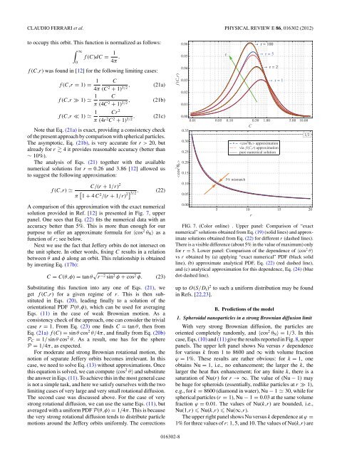
A comparison of this approximation with the exact numerical
solution provided in Ref. [12] is presented in Fig. 7, upper
panel. One sees that Eq. (22) fits the numerical data with an
accuracy better than 5%. This is more than enough for our
purpose to offer an approximate formula for 〈cos2 θN〉 as a
function of r; see below.
Next we use the fact that Jeffery orbits do not intersect on
the unit sphere. In other words, fixing C results in a relation
between θ and φ along an orbit. This relationship is obtained
by inverting Eq. (17b):
C = C(θ,φ) = tan θ r −2 sin 2 φ + cos 2 φ. (23)
Substituting this function into any one of Eqs. (21), we
get f (C,r) for a given regime of r. This is then substituted
in Eqs. (20), leading finally to a solution of the
orientational PDF P(θ,φ), which can be used for averaging
Eqs. (11) in the case of weak Brownian motion. As a
consistency check of the approach, one can consider the trivial
case r = 1. From Eq. (23) one finds C = tan θ, then from
Eq. (21a) f (C) = sin θ cos 2 θ/4π, and finally from Eq. (20b)
PC = 1/ sin θ cos 2 θ. As a result, one has for the sphere
P = 1/4π, as expected.
For moderate and strong Brownian rotational motion, the
notion of separate Jeffery orbits becomes irrelevant. In this
case, we need to solve Eq. (13) without approximations. Once
this equation is solved, we can compute 〈cos 2 θ〉 and substitute
the answer in Eqs. (11). To achieve this in the most general case
is not a simple task, and here we satisfy ourselves with the two
limiting cases of very large and very small rotational diffusion.
The second case was discussed above. For the case of very
strong rotational diffusion, we can use the same Eqs. (11),but
averaged with a uniform PDF P(θ,φ) = 1/4π. This is because
the very strong rotational diffusion tends to distribute particle
motions around the Jeffery orbits uniformly. The corrections
f C,r
cos 2 θ N
016302-8
0.06
0.05
0.04
0.03
0.02
0.01
r
r 100
r 5
r 2
r 1
0.00
0.01 0.05 0.10 0.50 1.00 5.00 10.00
C
0.35
1 3
0.30
0.25
0.20
0.15
0.10
0.05
0.00
cos 2 θN approximation
—– via f C,r approximation
—— pure numerical solution
5 mismatch
5 10 15 20
r
FIG. 7. (Color online) . Upper panel: Comparison of “exact
numerical” solutions obtained from Eq. (19) (solid lines) and approximate
solutions obtained from Eq. (22) for different r (dashed lines).
There is a visible difference (about 5% in the value of maximum) only
for r = 5. Lower panel: Comparison of the dependence of 〈cos 2 θ〉
vs r obtained by (a) applying “exact numerical” PDF (black solid
line), (b) approximate analytical PDF, Eq. (22) (red dashed line),
and (c) analytical approximation for this dependence, Eq. (24) (blue
dot-dashed line).
up to O(S/Dr) 2 to such a uniform distribution may be found
in Refs. [22,23].
B. Predictions of the model
1. Spheroidal nanoparticles in a strong Brownian diffusion limit
With very strong Brownian diffusion, the particles are
oriented completely randomly, and 〈cos2 θN〉 =1/3. In this
case, Eqs. (10) and (11) give the results reported in Fig. 8, upper
panels. The upper left panel shows Nu versus r dependence
for various k from 1 to 8600 and ∞ with volume fraction
ϕ = 1%. These results are rather obvious: for k = 1, one
obtains Nu = 1, i.e., no enhancement; the larger the k, the
larger the heat flux enhancement; for any finite k, there is a
saturation of Nu(r) forr→∞.Thevalueof(Nu−1) may
be huge for spheroids (essentially, rodlike particles at r ≫ 1),
e.g., for k = 8600 (diamond in water), Nu − 1 30, while for
spherical particles (r = 1), Nu − 1 = 0.03 at the same volume
fraction ϕ = 0.01. The values of Nu(k,r) are bounded, i.e.,
Nu(1,r) Nu(k,r) Nu(∞,r).
The upper right panel shows Nu versus k dependence at ϕ =
1% for three values of r: 1, 5, and 10. The values of Nu(k,r)are