Nonlinear Static and Dynamic Analysis of Steel Structures with ...
Nonlinear Static and Dynamic Analysis of Steel Structures with ...
Nonlinear Static and Dynamic Analysis of Steel Structures with ...

You also want an ePaper? Increase the reach of your titles
YUMPU automatically turns print PDFs into web optimized ePapers that Google loves.
Δθνικό Μεηζόβιο Πολσηετνείο<br />
Σρνιή Πνιηηηθώλ Μεραληθώλ<br />
Εξγαζηήξην Σηαηηθήο θαη Αληηζεηζκηθώλ Εξεπλώλ<br />
ΔΠΜΣ: Δνκνζηαηηθόο Σρεδηαζκόο θαη Αλάιπζε Καηαζθεπώλ<br />
Μη Γραμμική ηαηική και Γσναμική Ανάλσζη Μεηαλλικών<br />
Καηαζκεσών με Λεπηομερή Προζομοιώμαηα Πεπεραζμένφν<br />
ηοιτείφν<br />
Αποζηόλης Α. Βράκας<br />
Επηβιέπσλ: Μ. Παπαδξαθάθεο, Καζεγεηήο ΕΜΠ<br />
Αζήνα, 2011
National Technical University <strong>of</strong> Athens<br />
School <strong>of</strong> Civil Engineering<br />
Institute <strong>of</strong> Structural <strong>Analysis</strong> <strong>and</strong> Antiseismic Research<br />
M.Sc.: <strong>Analysis</strong> <strong>and</strong> Design <strong>of</strong> Earthquake Resistant <strong>Structures</strong> (ADERS)<br />
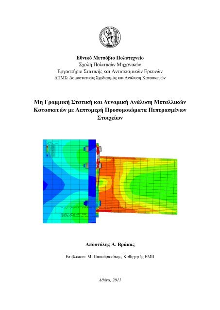
<strong>Nonlinear</strong> <strong>Static</strong> <strong>and</strong> <strong>Dynamic</strong> <strong>Analysis</strong> <strong>of</strong> <strong>Steel</strong> <strong>Structures</strong> <strong>with</strong><br />
Detailed Finite Element Models<br />
Apostolis A. Vrakas<br />
Supervisor: Pr<strong>of</strong>essor Manolis Papadrakakis<br />
Athens, 2011
National Technical University <strong>of</strong> Athens<br />
School <strong>of</strong> Civil Engineering<br />
Institute <strong>of</strong> Structural <strong>Analysis</strong> <strong>and</strong> Antiseismic Research<br />
M.Sc.: <strong>Analysis</strong> <strong>and</strong> Design <strong>of</strong> Earthquake Resistant <strong>Structures</strong> (ADERS)<br />
<strong>Nonlinear</strong> <strong>Static</strong> <strong>and</strong> <strong>Dynamic</strong> <strong>Analysis</strong> <strong>of</strong> <strong>Steel</strong> <strong>Structures</strong> <strong>with</strong> Detailed<br />
Finite Element Models<br />
postgraduate thesis<br />
by<br />
Apostolis A. Vrakas, Civil Engineer NTUA<br />
apostolis.vrakas@gmail.com<br />
Supervisor: Pr<strong>of</strong>essor Manolis Papadrakakis<br />
© 2011<br />
i
<strong>Nonlinear</strong> <strong>Static</strong> <strong>and</strong> <strong>Dynamic</strong> <strong>Analysis</strong> <strong>of</strong> <strong>Steel</strong> <strong>Structures</strong> <strong>with</strong> Detailed<br />
Finite Element Models<br />
Apostolis A. Vrakas<br />
Supervisor: Pr<strong>of</strong>essor Manolis Papadrakakis<br />
Institute <strong>of</strong> Structural <strong>Analysis</strong> <strong>and</strong> Antiseismic Research<br />
National Technical University <strong>of</strong> Athens<br />
Zografou Campus, Athens 15780, Greece<br />
apostolis.vrakas@gmail.com<br />
ABSTRACT<br />
The objective <strong>of</strong> this thesis is the nonlinear detailed finite element analysis <strong>of</strong> steel moment<br />
resisting frames <strong>with</strong> extended end-plate bolted beam-to-column joints. Firstly, the<br />
simulation <strong>of</strong> the joints is performed, using structural (beam <strong>and</strong> shell) <strong>and</strong> threedimensional<br />
continuum (eight-node hexahedral solid) elements. Material as well as<br />
geometric nonlinearities <strong>with</strong> contact between the appropriate components <strong>of</strong> the<br />
connections are taken into account. The moment-rotation (Μ-θ) response <strong>of</strong> characteristic<br />
joints, subjected to static loads, is calculated <strong>and</strong> compared <strong>with</strong> experimental results <strong>and</strong><br />
EC3 predictions for the validation <strong>of</strong> the corresponding numerical models.<br />
Then, multistory steel frames are examined <strong>with</strong> detailed modeling <strong>of</strong> their joints via<br />
structural elements according to the above study, capturing all types <strong>of</strong> nonlinearities.<br />
Frame members are modeled either <strong>with</strong> shell (full simulation) or <strong>with</strong> beam-column<br />
elements combined <strong>with</strong> proper compatibility constraints at the interfaces <strong>with</strong> the joints<br />
(hybrid simulation) accounting for the excessive computational effort required to perform<br />
nonlinear analyses <strong>with</strong> detailed finite element models. Pushover static <strong>and</strong> implicit directintegration<br />
dynamic analyses taking into consideration P-delta effects are performed<br />
demonstrating the effect <strong>of</strong> joints on the overall response <strong>of</strong> the structure. El Centro<br />
earthquake horizontal accelerogram is considered for the seismic excitation. In order to<br />
study the influence <strong>of</strong> the joints end-plate <strong>and</strong> bolts, parametric analyses are performed<br />
demonstrating the effect <strong>of</strong> each component on the overall behavior <strong>of</strong> the frame. Finally,<br />
stiffening <strong>of</strong> the joints <strong>with</strong> supplementary web plates takes place in order to examine the<br />
influence <strong>of</strong> the panel zone deformations.<br />
The detailed finite element discretization <strong>of</strong> the joint <strong>and</strong> frame models is produced<br />
automatically from their corresponding geometric description via appropriate code that has<br />
been developed, while Abaqus/St<strong>and</strong>ard s<strong>of</strong>tware is used for the numerical analyses.<br />
iii
Μη Γραμμική ηαηική και Γσναμική Ανάλσζη Μεηαλλικών<br />
Καηαζκεσών με Λεπηομερή Προζομοιώμαηα Πεπεραζμένφν ηοιτείφν<br />
Αποζηόλης Α. Βράκας<br />
Δπιβλέπφν: Μ. Παπαδρακάκης, Καθηγηηής ΔΜΠ<br />
Εξγαζηήξην Σηαηηθήο θαη Αληηζεηζκηθώλ Εξεπλώλ<br />
Εζληθό Μεηζόβην Πνιπηερλείν<br />
Πνιπηερλεηνύπνιε Ζσγξάθνπ, Αζήλα 15780, Ειιάδα<br />
apostolis.vrakas@gmail.com<br />
ΠΔΡΙΛΗΨΗ<br />
Σθνπόο απηήο ηεο εξγαζίαο είλαη ε κε γξακκηθή αλάιπζε κε ιεπηνκεξή πξνζνκνηώκαηα<br />
πεπεξαζκέλσλ ζηνηρείσλ κεηαζεηώλ κεηαιιηθώλ πιαηζίσλ απνηεινύκελσλ από<br />
θνριησηνύο θόκβνπο δνθνύ-ππνζηπιώκαηνο κε πξνεμέρνπζα κεησπηθή πιάθα. Αξρηθά,<br />
πξαγκαηνπνηείηαη πξνζνκνίσζε ησλ θόκβσλ: α) κε επηθαλεηαθά ζηνηρεία θειύθνπο ζε<br />
ζπλδπαζκό κε ξαβδσηά ζηνηρεία δνθνύ, θαη β) κε εμαεδξηθά-νθηαθνκβηθά ηξηζδηάζηαηα<br />
πεπεξαζκέλα ζηνηρεία. Λακβάλνληαη ππόςε ηόζν κε γξακκηθόηεηεο πιηθνύ όζν θαη<br />
γεσκεηξηθέο κε γξακκηθόηεηεο ζπκπεξηιακβαλνκέλσλ ησλ επαθώλ κεηαμύ ησλ δηαθόξσλ<br />
ζπζηαηηθώλ κεξώλ ησλ ζπλδέζεσλ. Υπνινγίδνληαη θακπύιεο ξνπήο-ζηξνθήο (Μ-θ)<br />
ραξαθηεξηζηηθώλ θόκβσλ ππνβαιιόκελσλ ζε ζηαηηθά θνξηία, θαη ζπγθξίλνληαη κε<br />
πεηξακαηηθά απνηειέζκαηα θαη πξνβιέςεηο ηνπ EC3 γηα ηελ απνηίκεζε ησλ δηαθόξσλ<br />
αξηζκεηηθώλ κνληέισλ.<br />
Αθνινπζεί ε αλάιπζε πνιπώξνθσλ κεηαιιηθώλ πιαηζίσλ κε ιεπηνκεξή πξνζνκνίσζε<br />
ησλ θόκβσλ ηνπο γηα ηελ εκθάληζε θάζε είδνπο κε γξακκηθήο ζπκπεξηθνξάο. Γηα ηα<br />
δνκηθά κέιε ρξεζηκνπνηνύληαη ηόζν πεπεξαζκέλα ζηνηρεία θειύθνπο (πιήξε κνληέια)<br />
όζν θαη ξαβδσηά ζηνηρεία δνθνύ-ππνζηπιώκαηνο κε ζεώξεζε θαηάιιεισλ θηλεκαηηθώλ<br />
εμαξηήζεσλ ζηηο δηεπηθάλεηεο (πβξηδηθά κνληέια) γηα ηελ αληηκεηώπηζε ηνπ κεγάινπ<br />
ππνινγηζηηθνύ θόζηνπο πνπ απαηηείηαη γηα ηελ πξαγκαηνπνίεζε κε γξακκηθώλ αλαιύζεσλ<br />
κε ιεπηνκεξή πξνζνκνηώκαηα πεπεξαζκέλσλ ζηνηρείσλ. Πξαγκαηνπνηνύληαη ηόζν κε<br />
γξακκηθέο ζηαηηθέο αλαιύζεηο ππό νξηδόληηα θνξηία (pushover) όζν θαη δπλακηθέο<br />
αλαιύζεηο ρξνλντζηνξίαο επηδεηθλύνληαο ηελ επηξξνή ησλ θόκβσλ ζηε ζπκπεξηθνξά ηνπ<br />
θνξέα. Ωο νξηδόληηα ζεηζκηθή δηέγεξζε ρξεζηκνπνηείηαη ν ζεηζκόο ηνπ El Centro.<br />
Πξαγκαηνπνηνύληαη παξακεηξηθέο αλαιύζεηο σο πξνο ηε κεησπηθή πιάθα θαη ηνπο θνριίεο<br />
κε ζθνπό λα θαλεί ε επηξξνή ησλ δηαθόξσλ ζπζηαηηθώλ κεξώλ ησλ θόκβσλ ζηελ<br />
θαζνιηθή απόθξηζε ηνπ θνξέα. Τέινο, εμεηάδεηαη ε επίδξαζε ηεο δηάηκεζεο ζηνλ θνξκό<br />
ηνπ ππνζηπιώκαηνο κέζσ ελίζρπζεο ηνπ κε πξόζζεηα ειάζκαηα.<br />
Η δηαθξηηνπνίεζε ησλ θόκβσλ θαη ησλ πιαηζίσλ ζε πεπεξαζκέλα ζηνηρεία γίλεηαη κέζσ<br />
θαηάιιεινπ ινγηζκηθνύ πνπ αλαπηύρζεθε. Γηα ηηο αξηζκεηηθέο αλαιύζεηο ρξεζηκνπνηείηαη<br />
ην Abaqus/St<strong>and</strong>ard.<br />
v
CONTENTS<br />
Abstract .................................................................................................................... iii<br />
Περίληυη .................................................................................................................... v<br />
Contents .................................................................................................................... vii<br />
Chapter 1 Design <strong>of</strong> <strong>Steel</strong> <strong>Structures</strong> <strong>with</strong> Eurocode 3 ................................ 1<br />
1.1 Materials .................................................................................................................... 1<br />
1.2 Classification <strong>of</strong> cross sections ................................................................................ 2<br />
1.3 Finite element methods <strong>of</strong> analysis .................................................................... 4<br />
1.3.1 General ........................................................................................................ 4<br />
1.3.2 Modeling ........................................................................................................ 5<br />
1.3.3 Use <strong>of</strong> imperfections ................................................................................ 5<br />
1.3.4 Material properties ................................................................................ 7<br />
1.3.5 Loads, limit state criteria <strong>and</strong> partial factors ............................................ 8<br />
1.4 Design <strong>of</strong> joints ........................................................................................................ 8<br />
1.4.1 Introduction ............................................................................................ 8<br />
1.4.2 Connections made <strong>with</strong> bolts .................................................................... 10<br />
1.4.3 Categories <strong>of</strong> bolted connections .................................................................... 10<br />
1.4.4 Positioning <strong>of</strong> holes for bolts <strong>and</strong> rivets ........................................................ 11<br />
1.4.5 Design resistance <strong>of</strong> individual fasteners ........................................................ 13<br />
1.4.6 <strong>Analysis</strong> <strong>of</strong> joints ............................................................................................ 15<br />
1.4.7 Classification <strong>of</strong> joints ................................................................................ 17<br />
1.4.8 Modeling <strong>of</strong> beam-to-column joints ........................................................ 18<br />
1.4.9 Design moment-rotation characteristic ........................................................ 21<br />
1.4.10 Basic components <strong>of</strong> a joint .................................................................... 21<br />
Chapter 2 Finite Element Modeling <strong>with</strong> ABAQUS/St<strong>and</strong>ard .................... 25<br />
2.1 Solid (continuum) elements ................................................................................ 25<br />
2.1.1 Choosing between first- <strong>and</strong> second-order elements ................................ 25<br />
2.1.2 Choosing between full- <strong>and</strong> reduced-integration elements ................................ 26<br />
2.1.3 Choosing between bricks/quadrilaterals <strong>and</strong> tetrahedra/triangles .................... 27<br />
2.1.4 Choosing between regular <strong>and</strong> hybrid elements ............................................ 27<br />
2.1.5 Incompatible mode elements .................................................................... 28<br />
2.1.6 Summary <strong>of</strong> recommendations for element usage ............................................ 28<br />
2.1.7 Naming convention ................................................................................ 29<br />
2.1.8 Node ordering <strong>and</strong> face numbering on elements ............................................ 30<br />
2.1.9 Numbering <strong>of</strong> integration points for output ............................................ 31<br />
2.2 Structural elements ............................................................................................ 32<br />
2.2.1 Beam elements ............................................................................................ 32<br />
2.2.2 Shell elements ............................................................................................ 34<br />
2.3 Interactions ........................................................................................................ 37<br />
2.3.1 Defining contact pairs ................................................................................ 37<br />
vii
2.3.2 Discretization <strong>of</strong> contact pair surfaces ........................................................ 37<br />
2.3.3 Contact tracking approaches .................................................................... 39<br />
2.3.4 Choosing the master <strong>and</strong> slave roles in a two-surface contact pair .................... 39<br />
2.3.5 Contact pressure-overclosure relationships ............................................ 40<br />
2.3.6 Contact constraint enforcement methods ............................................ 41<br />
2.3.7 Frictional behavior ................................................................................ 42<br />
2.3.8 Tied contact ............................................................................................ 44<br />
Chapter 3 <strong>Static</strong> <strong>Analysis</strong> <strong>of</strong> Beam-to-Column Joints ............................................ 45<br />
3.1 Introduction ........................................................................................................ 45<br />
3.2 Finite element modeling ............................................................................................ 45<br />
3.2.1 Simulation <strong>with</strong> shell elements .................................................................... 45<br />
3.2.2 Simulation <strong>with</strong> solid (continuum) elements ............................................ 46<br />
3.3 Experimental data ............................................................................................ 48<br />
3.4 Numerical results ............................................................................................ 49<br />
Chapter 4 <strong>Static</strong> <strong>Analysis</strong> <strong>of</strong> <strong>Steel</strong> Frames ........................................................ 61<br />
4.1 Introduction ........................................................................................................ 61<br />
4.2 Finite element modeling ............................................................................................ 61<br />
4.3 Frame A .................................................................................................................... 62<br />
4.4 Frame B .................................................................................................................... 68<br />
Chapter 5 <strong>Dynamic</strong> <strong>Analysis</strong> <strong>of</strong> <strong>Steel</strong> Frames ........................................................ 73<br />
5.1 Introduction ........................................................................................................ 73<br />
5.2 Finite element modeling ............................................................................................ 73<br />
5.3 Frame 1 .................................................................................................................... 76<br />
5.4 Frame 2 .................................................................................................................... 80<br />
Chapter 6 Conclusions ............................................................................................ 89<br />
References .................................................................................................................... 91<br />
viii
Chapter 1<br />
Design <strong>of</strong> <strong>Steel</strong> <strong>Structures</strong> <strong>with</strong> Eurocode 3<br />
1.1 Materials<br />
St<strong>and</strong>ard <strong>and</strong><br />
steel grade<br />
Nominal thickness <strong>of</strong> the element t [mm]<br />
t ≤ 40 mm 40 mm < t ≤ 80 mm<br />
fy [N/mm 2 ] fu [N/mm 2 ] fy [N/mm 2 ] fu [N/mm 2 ]<br />
EN 10025-2<br />
S 235 235 360 215 360<br />
S 275 275 430 255 410<br />
S 355 355 510 335 470<br />
S 450 440 550 410 550<br />
EN 10025-3<br />
S 275 N/NL 275 390 255 370<br />
S 355 N/NL 355 490 335 470<br />
S 420 N/NL 420 520 390 520<br />
S 460 N/NL 460 540 430 540<br />
EN 10025-4<br />
S 275 M/ML 275 370 255 360<br />
S 355 M/ML 355 470 335 450<br />
S 420 M/ML 420 520 390 500<br />
S 460 M/ML 460 540 430 530<br />
EN 10025-5<br />
S 235 W 235 360 215 340<br />
S 355 W 355 510 335 490<br />
EN 10025-6<br />
S 460<br />
Q/QL/QL1<br />
460 570 440 550<br />
Table 1.1: Nominal values <strong>of</strong> yield strength fy <strong>and</strong> ultimate tensile strength fu for hot rolled<br />
structural steel<br />
The material coefficients to be adopted in calculations for the structural steels should be<br />
taken as follows:<br />
– Modulus <strong>of</strong> elasticity E = 210 000 N/mm 2<br />
– Shear modulus G = E / 2(1+v) = 81 000 N/mm²<br />
– Poisson’s ratio in elastic stage v = 0.30<br />
– Coefficient <strong>of</strong> linear thermal expansion 12 x 10 -6 per o C (for T ≤ 100 o C)<br />
1
Chapter 1 Design <strong>of</strong> steel structures <strong>with</strong> Eurocode 3<br />
The bilinear stress-strain relationship indicated in Figure 1.1 may be used for the grades <strong>of</strong><br />
structural steel specified above. Alternatively, a more precise relationship may be adopted,<br />
as described in section 1.3.<br />
1.2 Classification <strong>of</strong> cross sections<br />
2<br />
Fig. 1.1: Bilinear stress-strain relationship<br />
The role <strong>of</strong> cross section classification is to identify the extent to which the resistance <strong>and</strong><br />
rotation capacity <strong>of</strong> cross sections is limited by its local buckling resistance.<br />
(1) Four classes <strong>of</strong> cross-sections are defined, as follows:<br />
– Class 1: cross-sections are those which can form a plastic hinge <strong>with</strong> the rotation<br />
capacity required from plastic analysis <strong>with</strong>out reduction <strong>of</strong> the resistance.<br />
– Class 2: cross-sections are those which can develop their plastic moment resistance,<br />
but have limited rotation capacity because <strong>of</strong> local buckling.<br />
– Class 3: cross-sections are those in which the stress in the extreme compression fibre<br />
<strong>of</strong> the steel member assuming an elastic distribution <strong>of</strong> stresses can reach the yield<br />
strength, but local buckling is liable to prevent development <strong>of</strong> the plastic moment<br />
resistance.<br />
– Class 4: cross-sections are those in which local buckling will occur before the<br />
attainment <strong>of</strong> yield stress in one or more parts <strong>of</strong> the cross-section.<br />
(2) In Class 4 cross sections effective widths may be used to make the necessary<br />
allowances for reductions in resistance due to the effects <strong>of</strong> local buckling, see EN<br />
1993-1-5, 5.2.2.<br />
(3) The classification <strong>of</strong> a cross-section depends on the width to thickness ratio <strong>of</strong> the parts<br />
subject to compression.<br />
(4) Compression parts include every part <strong>of</strong> a cross-section which is either totally or<br />
partially in compression under the load combination considered.<br />
(5) The various compression parts in a cross-section (such as a web or flange) can, in<br />
general, be in different classes.<br />
(6) A cross-section is classified according to the highest (least favorable) class <strong>of</strong> its<br />
compression parts. Exceptions are specified in EN 1993-1-1, 6.2.1(10), 6.2.2.4(1).<br />
(7) Alternatively the classification <strong>of</strong> a cross-section may be defined by quoting both the<br />
flange classification <strong>and</strong> the web classification.<br />
(8) The limiting proportions for Class 1, 2, <strong>and</strong> 3 compression parts should be obtained<br />
from Table 1.2. A part which fails to satisfy the limits for Class 3 should be taken as<br />
Class 4.
Chapter 1 Design <strong>of</strong> steel structures <strong>with</strong> Eurocode 3<br />
Stress<br />
distribution<br />
in parts<br />
(compression<br />
positive)<br />
4<br />
3 c / t 124<br />
c / t 42<br />
42<br />
when 1:<br />
c / t <br />
0,<br />
67 0,<br />
33<br />
when 1<br />
*)<br />
: c / t 62<br />
( 1<br />
) ( <br />
)<br />
235/<br />
f y<br />
fy<br />
<br />
235<br />
1,00<br />
275<br />
0,92<br />
355<br />
0,81<br />
420<br />
0,75<br />
460<br />
0,71<br />
*)<br />
where ς ≤ -1 applies where either the compression stress ζ < fy or the tensile strain εy > fy/E<br />
Table 1.2: Maximum width-to-thickness ratios for compression parts<br />
1.3 Finite element methods <strong>of</strong> analysis<br />
1.3.1 General<br />
The choice <strong>of</strong> the FE-method depends on the problem to be analysed <strong>and</strong> based on the<br />
following assumptions:<br />
No Material<br />
behavior<br />
f y<br />
-<br />
+<br />
f y<br />
c/2<br />
c<br />
Geometric<br />
behavior<br />
Imperfections Example <strong>of</strong> use<br />
1 linear linear no elastic shear lag effect, elastic resistance<br />
2 nonlinear linear no plastic resistance in ULS<br />
3 linear nonlinear no critical plate buckling load<br />
4 linear nonlinear yes elastic plate buckling resistance<br />
5 nonlinear nonlinear yes elastic-plastic resistance in ULS<br />
Table 1.3: Assumptions for FE-methods<br />
Use<br />
In using FEM for design, special care should be taken to:<br />
– the modeling <strong>of</strong> the structural component <strong>and</strong> its boundary conditions;<br />
– the choice <strong>of</strong> s<strong>of</strong>tware <strong>and</strong> documentation;<br />
– the use <strong>of</strong> imperfections;<br />
– the modeling <strong>of</strong> material properties;<br />
– the modeling <strong>of</strong> loads;<br />
– the modeling <strong>of</strong> limit state criteria;<br />
– the partial factors to be applied.<br />
+<br />
f y<br />
c<br />
-<br />
f y<br />
+<br />
f y<br />
c
Design <strong>of</strong> steel structures <strong>with</strong> Eurocode 3 Chapter 1<br />
1.3.2 Modeling<br />
(1) The choice <strong>of</strong> FE-models (shell models or volume models) <strong>and</strong> the size <strong>of</strong> mesh<br />
determine the accuracy <strong>of</strong> results. For validation sensitivity checks <strong>with</strong> successive<br />
refinement may be carried out.<br />
(2) The FE-modeling may be carried out either for:<br />
– the component as a whole or<br />
– a substructure as a part <strong>of</strong> the whole structure.<br />
NOTE: An example for a component could be the web <strong>and</strong>/or the bottom plate <strong>of</strong><br />
continuous box girders in the region <strong>of</strong> an intermediate support where the bottom plate is<br />
in compression. An example for a substructure could be a subpanel <strong>of</strong> a bottom plate<br />
subject to biaxial stresses.<br />
(3) The boundary conditions for supports, interfaces <strong>and</strong> applied loads should be chosen<br />
such that results obtained are conservative.<br />
(4) Geometric properties should be taken as nominal.<br />
(5) All imperfections should be based on the shapes <strong>and</strong> amplitudes <strong>of</strong> section 1.3.5.<br />
(6) Material properties should conform to section 1.3.6.<br />
Choice <strong>of</strong> s<strong>of</strong>tware <strong>and</strong> documentation<br />
(1) The s<strong>of</strong>tware should be suitable for the task <strong>and</strong> be proven reliable.<br />
NOTE: Reliability can be proven by appropriate benchmark tests.<br />
(2) The mesh size, loading, boundary conditions <strong>and</strong> other input data as well as the output<br />
should be documented in a way that they can be reproduced by third parties.<br />
1.3.3 Use <strong>of</strong> imperfections<br />
(1) Where imperfections need to be included in the FE-model these imperfections should<br />
include both geometric <strong>and</strong> structural imperfections.<br />
(2) Unless a more refined analysis <strong>of</strong> the geometric imperfections <strong>and</strong> the structural<br />
imperfections is carried out, equivalent geometric imperfections may be used.<br />
NOTE 1: Geometric imperfections may be based on the shape <strong>of</strong> the critical plate buckling<br />
modes <strong>with</strong> amplitudes given in the National Annex. 80% <strong>of</strong> the geometric fabrication<br />
tolerances is recommended.<br />
NOTE 2: Structural imperfections in terms <strong>of</strong> residual stresses may be represented by a<br />
stress pattern from the fabrication process <strong>with</strong> amplitudes equivalent to the mean<br />
(expected) values.<br />
(3) The direction <strong>of</strong> the applied imperfection should be such that the lowest resistance is<br />
obtained.<br />
(4) For applying equivalent geometric imperfections Table 1.4 <strong>and</strong> Figure 1.2 may be used.<br />
Type <strong>of</strong><br />
imperfection<br />
Component Shape Magnitude<br />
global member <strong>with</strong> length l bow<br />
see EN 1993-1-1,<br />
Table 5.1<br />
global longitudinal stiffener <strong>with</strong> length a bow min (a/400, b/400)<br />
local<br />
panel or subpanel <strong>with</strong> short span<br />
a or b<br />
buckling shape min (a/200, b/200)<br />
local stiffener or flange subject to twist bow twist 1 / 50<br />
Table 1.4: Equivalent geometric imperfections<br />
5
Chapter 1 Design <strong>of</strong> steel structures <strong>with</strong> Eurocode 3<br />
6<br />
Type <strong>of</strong><br />
imperfection<br />
global member<br />
<strong>with</strong> length l<br />
global<br />
longitudinal<br />
stiffener <strong>with</strong><br />
length a<br />
local panel or<br />
subpanel<br />
local stiffener or<br />
flange subject to<br />
twist<br />
b<br />
Component<br />
e 0y<br />
Fig. 1.2: Modeling <strong>of</strong> equivalent geometric imperfections<br />
<br />
e 0z<br />
b a<br />
e 0w<br />
a<br />
b<br />
a<br />
b<br />
__ 1<br />
50<br />
e 0w<br />
e 0w<br />
a
Design <strong>of</strong> steel structures <strong>with</strong> Eurocode 3 Chapter 1<br />
(5) In combining imperfections a leading imperfection should be chosen <strong>and</strong> the<br />
accompanying imperfections may have their values reduced to 70%.<br />
NOTE 1: Any type <strong>of</strong> imperfection should be taken as the leading imperfection <strong>and</strong> the<br />
others may be taken as the accompanying imperfections.<br />
NOTE 2: Equivalent geometric imperfections may be substituted by the appropriate<br />
fictitious forces acting on the member.<br />
1.3.4 Material properties<br />
(1) Material properties should be taken as characteristic values.<br />
(2) Depending on the accuracy <strong>and</strong> the allowable strain required for the analysis, the<br />
following assumptions for the material behaviour may be used, see Figure 1.3:<br />
a) elastic-plastic <strong>with</strong>out strain hardening;<br />
b) elastic-plastic <strong>with</strong> a nominal plateau slope;<br />
c) elastic-plastic <strong>with</strong> linear strain hardening;<br />
d) true stress-strain curve modified from the test results as follows:<br />
ζtrue = ζ (1+ε)<br />
εtrue = ln (1+ε)<br />
Model<br />
<strong>with</strong> yielding<br />
plateau<br />
<strong>with</strong> strainhardening<br />
ζ<br />
f y<br />
ζ<br />
f y<br />
tan -1 (E)<br />
tan -1 (E)<br />
α) a) β) b)<br />
γ) c)<br />
ε<br />
ε<br />
tan -1 (E/100)<br />
ζ<br />
f y 1<br />
tan -1 (E)<br />
1 tan -1 (E/10000)<br />
(or similarly small value)<br />
ζ<br />
f y<br />
1<br />
tan -1 (E)<br />
Fig.1.3: Modeling <strong>of</strong> material behavior<br />
2<br />
δ) d)<br />
1 true stress-strain curve<br />
2 stress-strain curve from tests<br />
ε<br />
ε<br />
7
Chapter 1 Design <strong>of</strong> steel structures <strong>with</strong> Eurocode 3<br />
1.3.5 Loads, limit state criteria <strong>and</strong> partial factors<br />
Loads<br />
(1) The loads applied to the structures should include relevant load factors <strong>and</strong> load<br />
combination factors. For simplicity a single load multiplier a may be used.<br />
Limit state criteria<br />
(1) The ultimate limit state criteria should be used as follows:<br />
1. for structures susceptible to buckling: attainment <strong>of</strong> the maximum load.<br />
2. for regions subjected to tensile stresses: attainment <strong>of</strong> a limiting value <strong>of</strong> the principal<br />
membrane strain.<br />
NOTE 1: The National Annex may specify the limiting <strong>of</strong> principal strain. A value <strong>of</strong> 5%<br />
is recommended.<br />
NOTE 2: Other criteria may be used, e.g. attainment <strong>of</strong> the yielding criterion or limitation<br />
<strong>of</strong> the yielding zone.<br />
Partial factors<br />
(1) The load magnification factor au to the ultimate limit state should be sufficient to<br />
achieve the required reliability.<br />
(2) The magnification factor au should consist <strong>of</strong> two factors as follows:<br />
1. a1 to cover the model uncertainty <strong>of</strong> the FE-modeling used. It should be obtained from<br />
evaluations <strong>of</strong> test calibrations;<br />
2. a2 to cover the scatter <strong>of</strong> the loading <strong>and</strong> resistance models. It may be taken as γΜ1 if<br />
instability governs <strong>and</strong> γΜ2 if fracture governs.<br />
(3) It should be verified that: au > a1 a2<br />
NOTE: The National Annex may give information on γΜ1 <strong>and</strong> γΜ2. The use <strong>of</strong> γΜ1 <strong>and</strong> γΜ2<br />
as specified in the relevant parts <strong>of</strong> EN 1993 is recommended.<br />
1.4 Design <strong>of</strong> joints<br />
1.4.1 Introduction<br />
Joint is defined as the zone where two or more members are interconnected. For design<br />
purposes it is the assembly <strong>of</strong> all the basic components required to represent the behaviour<br />
during the transfer <strong>of</strong> the relevant internal forces <strong>and</strong> moments between the connected<br />
members. A beam-to-column joint consists <strong>of</strong> a web panel <strong>and</strong> either one connection<br />
(single sided joint configuration) or two connections (double sided joint configuration), see<br />
Figure 1.4.<br />
Connection is defined as the location at which two or more elements meet. For design<br />
purposes it is the assembly <strong>of</strong> the basic components required to represent the behaviour<br />
during the transfer <strong>of</strong> the relevant internal forces <strong>and</strong> moments at the connection.<br />
8
Design <strong>of</strong> steel structures <strong>with</strong> Eurocode 3 Chapter 1<br />
1<br />
3<br />
2<br />
Joint = web panel in shear + connection Left joint = web panel in shear + left connection<br />
Right joint = web panel in shear + right connection<br />
1<br />
1<br />
a)Single-sided joint configuration b)Double-sided joint configuration<br />
1 web panel in shear<br />
2 connection<br />
3 components (e.g. bolts, endplate)<br />
Fig.1.4: Parts <strong>of</strong> a beam-to-column joint configuration<br />
3 3<br />
a) Major axis joint configurations<br />
2<br />
2<br />
5<br />
5<br />
2<br />
4<br />
1<br />
1 Single-sided beam-to<br />
column joint<br />
configuration;<br />
2 Double-sided beam-tocolumn<br />
joint<br />
configuration;<br />
Double-sided beam-to-column Double-sided beam-to-column<br />
joint configuration joint configuration<br />
b) Minor-axis joint configurations (to be used only for balanced moments Mb1,Ed = Mb2,Ed)<br />
3<br />
3 Beam splice;<br />
4 Column splice;<br />
5 Column base<br />
2<br />
9
Chapter 1 Design <strong>of</strong> steel structures <strong>with</strong> Eurocode 3<br />
Fig.1.5: Joint configurations<br />
1.4.2 Connections made <strong>with</strong> bolts<br />
The yield strength fyb <strong>and</strong> the ultimate tensile strength fub for bolt classes 4.6, 5.6, 6.8, 8.8<br />
<strong>and</strong> 10.9 are given in Table 1.5. These values should be adopted as characteristic values in<br />
design calculations.<br />
10<br />
Bolt class 4.6 5.6 6.8 8.8 10.9<br />
fyb (N/mm 2 ) 240 300 480 640 900<br />
fub (N/mm 2 ) 400 500 600 800 1000<br />
Table 1.5: Nominal values <strong>of</strong> the yield strength fyb <strong>and</strong> the ultimate tensile strength fub for<br />
bolts<br />
Only bolt assemblies <strong>of</strong> classes 8.8 <strong>and</strong> 10.9 conforming to the requirements given in 2.8<br />
Reference St<strong>and</strong>ards: Group 4 for High Strength Structural Bolting <strong>with</strong> controlled<br />
tightening in accordance <strong>with</strong> the requirements in 2.8 Reference St<strong>and</strong>ards: Group 7 may<br />
be used as preloaded bolts.<br />
1.4.3 Categories <strong>of</strong> bolted connections<br />
Shear connections<br />
Bolted connections loaded in shear should be designed as one <strong>of</strong> the following:<br />
a) Category A: Bearing type<br />
In this category bolts from class 4.6 up to <strong>and</strong> including class 10.9 should be used.<br />
No preloading <strong>and</strong> special provisions for contact surfaces are required. The design<br />
ultimate shear load should not exceed the design shear resistance nor the design<br />
bearing resistance.<br />
b) Category B: Slip-resistant <strong>and</strong> serviceability limit state<br />
In this category preloaded bolts should be used. Slip should not occur at the<br />
serviceability limit state. The design serviceability shear load should not exceed the<br />
design slip resistance. The design ultimate shear load should not exceed the design<br />
shear resistance nor the design bearing resistance.<br />
c) Category C: Slip-resistant at ultimate limit state<br />
In this category preloaded bolts should be used. Slip should not occur at the<br />
ultimate limit state. The design ultimate shear load should not exceed the design<br />
slip resistance nor the design bearing resistance. In addition for a connection in<br />
tension, the design plastic resistance <strong>of</strong> the net cross-section at bolt holes Nnet,Rd,<br />
(see 6.2 <strong>of</strong> EN 1993-1-1), should be checked, at the ultimate limit state.<br />
The design checks for these connections are summarized in Table 1.6.<br />
Tension connections<br />
Bolted connection loaded in tension should be designed as one <strong>of</strong> the following:<br />
a) Category D: non-preloaded<br />
In this category bolts from class 4.6 up to <strong>and</strong> including class 10.9 should be used.<br />
No preloading is required. This category should not be used where the connections<br />
are frequently subjected to variations <strong>of</strong> tensile loading. However, they may be<br />
used in connections designed to resist normal wind loads.
Design <strong>of</strong> steel structures <strong>with</strong> Eurocode 3 Chapter 1<br />
b) Category E: preloaded<br />
In this category preloaded 8.8 <strong>and</strong> 10.9 bolts <strong>with</strong> controlled tightening in<br />
conformity <strong>with</strong> 2.8 Reference St<strong>and</strong>ards: Group 7 should be used.<br />
The design checks for these connections are summarized in Table 1.6.<br />
Category Criteria Remarks<br />
Shear connections<br />
A<br />
bearing type<br />
B<br />
slip-resistant at<br />
serviceability<br />
C<br />
slip-resistant at<br />
ultimate<br />
D<br />
non-preloaded<br />
E<br />
preloaded<br />
Fv,Ed ≤ Fv,Rd<br />
Fv,Ed ≤ Fb,Rd<br />
Fv,Ed.ser ≤ Fs,Rd,ser<br />
Fv,Ed ≤ Fv,Rd<br />
Fv,Ed ≤ Fb,Rd<br />
Fv,Ed ≤ Fs,Rd<br />
Fv,Ed ≤ Fb,Rd<br />
Fv,Ed ≤ Nnet,Rd<br />
Ft,Ed ≤ Ft,Rd<br />
Ft,Ed ≤ Bp,Rd<br />
Ft,Ed ≤ Ft,Rd<br />
Ft,Ed ≤ Bp,Rd<br />
Tension connections<br />
No preloading required.<br />
Bolt classes from 4.6 to 10.9 may be used.<br />
Preloaded 8.8 or 10.9 bolts should be used.<br />
For slip resistance at serviceability see EN<br />
1993-1-8, 3.9.<br />
Preloaded 8.8 or 10.9 bolts should be used.<br />
For slip resistance at ultimate see EN 1993-<br />
1-8, 3.9.<br />
Nnet,Rd see EN 1993-1-1.<br />
No preloading required.<br />
Bolt classes from 4.6 to 10.9 may be used.<br />
Bp,Rd see Table 1.8.<br />
Preloaded 8.8 or 10.9 bolts should be used.<br />
Bp,Rd see Table 1.8.<br />
The design tensile force Ft,Ed should include any force due to prying action, see EN<br />
1993-1-8, 3.11. Bolts subjected to both shear force <strong>and</strong> tensile force should also satisfy<br />
the criteria given in Table 1.8.<br />
Table 1.6: Categories <strong>of</strong> bolted connections<br />
1.4.4 Positioning <strong>of</strong> holes for bolts <strong>and</strong> rivets<br />
Minimum <strong>and</strong> maximum spacing <strong>and</strong> end <strong>and</strong> edge distances for bolts <strong>and</strong> rivets are given<br />
in Table 1.7.<br />
Distances <strong>and</strong><br />
spacings,<br />
see Figure 1.6<br />
Minimum Maximum<br />
1) 2) 3)<br />
<strong>Structures</strong> made from steels conforming to<br />
EN 10025 except steels conforming to EN<br />
10025-5<br />
<strong>Steel</strong> exposed to the<br />
weather or other<br />
corrosive influences<br />
<strong>Steel</strong> not exposed to<br />
the weather or other<br />
corrosive influences<br />
<strong>Structures</strong> made from<br />
steels conforming to<br />
EN 10025-5<br />
<strong>Steel</strong> used<br />
unprotected<br />
End distance e1 1,2d0 4t + 40 mm The larger <strong>of</strong><br />
8t or 125 mm<br />
Edge distance e2 1,2d0 4t + 40 mm The larger <strong>of</strong><br />
Distance e3<br />
in slotted holes<br />
1,5d0 4)<br />
8t or 125 mm<br />
11
Chapter 1 Design <strong>of</strong> steel structures <strong>with</strong> Eurocode 3<br />
Distance e4<br />
in slotted holes<br />
Spacing p1 2,2d0 The smaller <strong>of</strong><br />
14t or 200 mm<br />
12<br />
1,5d0 4)<br />
Spacing p1,0 The smaller <strong>of</strong><br />
14t or 200 mm<br />
Spacing p1,i The smaller <strong>of</strong><br />
28t or 400 mm<br />
The smaller <strong>of</strong><br />
14t or 200 mm<br />
The smaller <strong>of</strong><br />
14tmin or 175 mm<br />
Spacing p2 5) 2,4d0 The smaller <strong>of</strong> The smaller <strong>of</strong> The smaller <strong>of</strong><br />
14t or 200 mm 14t or 200 mm 14tmin or 175 mm<br />
1) Maximum values for spacings, edge <strong>and</strong> end distances are unlimited, except in the following<br />
cases:<br />
– for compression members in order to avoid local buckling <strong>and</strong> to prevent corrosion in exposed<br />
members <strong>and</strong>;<br />
– for exposed tension members to prevent corrosion.<br />
2) The local buckling resistance <strong>of</strong> the plate in compression between the fasteners should be<br />
calculated according to EN 1993-1-1 using 0,6 pi as buckling length. Local buckling between the<br />
fasteners need not to be checked if p1/t is smaller than 9 ε. The edge distance should not exceed the<br />
local buckling requirements for an outst<strong>and</strong> element in the compression members, see EN 1993-1-<br />
1. The end distance is not affected by this requirement.<br />
3) t is the thickness <strong>of</strong> the thinner outer connected part.<br />
4) The dimensional limits for slotted holes are given in 2.8 Reference St<strong>and</strong>ards: Group 7.<br />
5) For staggered rows <strong>of</strong> fasteners a minimum line spacing <strong>of</strong> p2 = 1,2d0 may be used, provided that<br />
the minimum distance, L, between any two fasteners is greater than 2,4d0, see Figure 1.6 b).<br />
Table 1.7: Minimum <strong>and</strong> maximum spacing, end <strong>and</strong> edge distances<br />
Staggered rows <strong>of</strong> fasteners<br />
a) Symbols for spacing <strong>of</strong> fasteners b) Symbols for staggered spacing<br />
p1 ≤ 14 t <strong>and</strong> ≤ 200 mm p2 ≤ 14 t <strong>and</strong> ≤ 200 mm p1,0 ≤ 14 t <strong>and</strong> ≤ 200 mm p1,i ≤ 28 t <strong>and</strong> ≤ 400 mm<br />
1 outer row 2 inner row<br />
c) Staggered spacing – compression d) Spacing in tension members
Design <strong>of</strong> steel structures <strong>with</strong> Eurocode 3 Chapter 1<br />
e) End <strong>and</strong> edge distances for slotted holes<br />
Fig. 1.6: Symbols for end <strong>and</strong> edge distances <strong>and</strong> spacing <strong>of</strong> fasteners<br />
1.4.5 Design resistance <strong>of</strong> individual fasteners<br />
Failure mode Bolts Rivets<br />
Shear resistance per shear<br />
plane<br />
Fv,Rd =<br />
Bearing resistance 1), 2), 3) Fb,Rd =<br />
<br />
v<br />
f<br />
<br />
ub<br />
M 2<br />
A<br />
- where the shear plane passes through the<br />
threaded portion <strong>of</strong> the bolt (A is the tensile<br />
stress area <strong>of</strong> the bolt As):<br />
- for classes 4.6, 5.6 <strong>and</strong> 8.8:<br />
av = 0,6<br />
- for classes 4.8, 5.8, 6.8 <strong>and</strong> 10.9:<br />
av = 0,5<br />
- where the shear plane passes through the<br />
unthreaded portion <strong>of</strong> the bolt (A is the gross<br />
cross section <strong>of</strong> the bolt): av = 0,6<br />
k a f d t<br />
1<br />
b<br />
<br />
u<br />
M 2<br />
where αb is the smallest <strong>of</strong> αd or<br />
f<br />
f<br />
ub<br />
u<br />
or 1,0;<br />
In the direction <strong>of</strong> load transfer:<br />
e1<br />
- for end bolts: αd = , for inner bolts: αd =<br />
3d<br />
Perpendicular to the direction <strong>of</strong> load transfer:<br />
0<br />
0<br />
Fv,Rd =<br />
p1<br />
1<br />
<br />
d 4<br />
3 0<br />
e2<br />
- for edge bolts: k1 is the smallest <strong>of</strong> 2,<br />
8 1,<br />
7 or 2,5<br />
d<br />
0,<br />
6<br />
p2<br />
- for inner bolts: k1 is the smallest <strong>of</strong> 1,<br />
4 1,<br />
7 or 2,5<br />
d<br />
0<br />
f<br />
<br />
ur A0<br />
M 2<br />
13
Chapter 1 Design <strong>of</strong> steel structures <strong>with</strong> Eurocode 3<br />
Tension resistance 2)<br />
14<br />
Ft,Rd =<br />
k<br />
2<br />
ub s A f<br />
<br />
M 2<br />
where k2 = 0,63 for countersunk bolt,<br />
otherwise k2 = 0,9.<br />
Ft,Rd =<br />
Punching shear resistance Bp,Rd = 0,6 π dm tp fu / γM2 No check needed<br />
Combined shear <strong>and</strong><br />
tension<br />
F<br />
F<br />
v,<br />
Ed<br />
v,<br />
Rd<br />
Ft<br />
, Ed<br />
<br />
1 , 4 Ft<br />
,<br />
Rd<br />
<br />
1,<br />
0<br />
0,<br />
6<br />
f<br />
<br />
ur 0 A<br />
1) The bearing resistance Fb,Rd for bolts<br />
– in oversized holes is 0,8 times the bearing resistance for bolts in normal holes.<br />
– in slotted holes, where the longitudinal axis <strong>of</strong> the slotted hole is perpendicular to the direction<br />
<strong>of</strong> the force transfer, is 0,6 times the bearing resistance for bolts in round, normal holes.<br />
2) For countersunk bolt:<br />
– the bearing resistance Fb,Rd should be based on a plate thickness t equal to the thickness <strong>of</strong> the<br />
connected plate minus half the depth <strong>of</strong> the countersinking.<br />
– for the determination <strong>of</strong> the tension resistance Ft,Rd the angle <strong>and</strong> depth <strong>of</strong> countersinking should<br />
conform <strong>with</strong> 2.8 Reference St<strong>and</strong>ards: Group 4, otherwise the tension resistance Ft,Rd should be<br />
adjusted accordingly.<br />
3) When the load on a bolt is not parallel to the edge, the bearing resistance may be verified<br />
separately for the bolt load components parallel <strong>and</strong> normal to the end.<br />
Table 1.8: Design resistance for individual fasteners subjected to shear <strong>and</strong>/or tension<br />
Design <strong>of</strong> steel structures <strong>with</strong> Eurocode 3 Chapter 1<br />
1.4.6 <strong>Analysis</strong> <strong>of</strong> joints<br />
General<br />
(1) The effects <strong>of</strong> the behaviour <strong>of</strong> the joints on the distribution <strong>of</strong> internal forces <strong>and</strong><br />
moments <strong>with</strong>in a structure, <strong>and</strong> on the overall deformations <strong>of</strong> the structure, should<br />
generally be taken into account, but where these effects are sufficiently small they may be<br />
neglected.<br />
(2) To identify whether the effects <strong>of</strong> joint behaviour on the analysis need be taken into<br />
account, a distinction may be made between three simplified joint models as follows:<br />
– simple, in which the joint may be assumed not to transmit bending moments;<br />
– continuous, in which the behaviour <strong>of</strong> the joint may be assumed to have no effect on the<br />
analysis;<br />
– semi-continuous, in which the behaviour <strong>of</strong> the joint needs to be taken into account in the<br />
analysis.<br />
(3) The appropriate type <strong>of</strong> joint model should be determined from Table 1.9, depending<br />
on the classification <strong>of</strong> the joint <strong>and</strong> on the chosen method <strong>of</strong> analysis.<br />
(4) The design moment-rotation characteristic <strong>of</strong> a joint used in the analysis may be<br />
simplified by adopting any appropriate curve, including a linearized approximation (e.g.<br />
bi-linear or tri-linear), provided that the approximate curve lies wholly below the design<br />
moment-rotation characteristic.<br />
Method <strong>of</strong><br />
global analysis<br />
Classification <strong>of</strong> joints<br />
Elastic Nominally pinned Rigid Semi-rigid<br />
Rigid-plastic Nominally pinned Full-strength Partial-strength<br />
Elastic-plastic Nominally pinned<br />
Rigid <strong>and</strong> fullstrength<br />
Semi-rigid <strong>and</strong> partial strength<br />
Semi-rigid <strong>and</strong> full-strength<br />
Rigid <strong>and</strong> partial-strength<br />
Type <strong>of</strong> joint<br />
model<br />
Simple Continuous Semi-continuous<br />
Table 1.9: Type <strong>of</strong> joint model<br />
Elastic global analysis<br />
(1) The joints should be classified according to their rotational stiffness, see 1.4.7.<br />
(2) The joints shall have sufficient strength to transmit the forces <strong>and</strong> moments acting at<br />
the joints resulting from the analysis.<br />
(3) In the case <strong>of</strong> a semi-rigid joint, the rotational stiffness Sj corresponding to the bending<br />
moment Mj,Ed should generally be used in the analysis. If Mj,Ed does not exceed 2/3 Mj,Rd<br />
the initial rotational stiffness Sj,ini may be taken in the global analysis, see Figure 1.10(a).<br />
(4) As a simplification to (3), the rotational stiffness may be taken as Sj,ini/ε in the<br />
analysis, for all values <strong>of</strong> the moment Mj,Ed, as shown in Figure 1.10(b), where ε is the<br />
stiffness modification coefficient from Table 1.10.<br />
(5) For joints connecting H or I sections Sj is given in EN 1993-1-8, 6.3.1.<br />
15
Chapter 1 Design <strong>of</strong> steel structures <strong>with</strong> Eurocode 3<br />
16<br />
M j,Rd<br />
2/3 M j,Rd<br />
M j,Ed<br />
M j<br />
S j,ini<br />
a) Mj,Ed ≤ 2/3 Mj,Rd b) Mj,Ed ≤ Mj,Rd<br />
Fig. 1.10: Rotational stiffness to be used in elastic global analysis<br />
Type <strong>of</strong> connection Beam-to-column<br />
joints<br />
<br />
Other types <strong>of</strong> joints<br />
(beam-to-beam<br />
joints, beam splices,<br />
column base joints)<br />
Welded 2 3<br />
Bolted end-plate 2 3<br />
Bolted flange cleats 2 3,5<br />
Base plates - 3<br />
Table 1.10: Stiffness modification coefficient ε<br />
Rigid-plastic global analysis<br />
(1) The joints should be classified according to their strength, see 1.4.7.<br />
(2) For joints connecting H or I sections Mj,Rd is given in EN 1993-1-8, 6.2.<br />
(3) For joints connecting hollow sections the method given in EN 1993-1-8, section 7 may<br />
be used.<br />
(4) The rotation capacity <strong>of</strong> a joint shall be sufficient to accommodate the rotations<br />
resulting from the analysis.<br />
(5) For joints connecting H or I sections the rotation capacity should be checked according<br />
to EN 1993-1-8, 6.4.<br />
Elastic-plastic global analysis<br />
(1) The joints should be classified according to both stiffness <strong>and</strong> strength (see 1.4.7).<br />
(2) For joints connecting H or I sections Mj,Rd is given in EN 1993-1-8, 6.2, Sj is given in<br />
EN 1993-1-8, 6.3.1 <strong>and</strong> θCd is given in EN 1993-1-8, 6.4.<br />
(3) For joints connecting hollow sections the method given in EN 1993-1-8, section 7 may<br />
be used.<br />
(4) The moment rotation characteristic <strong>of</strong> the joints should be used to determine the<br />
distribution <strong>of</strong> internal forces <strong>and</strong> moments.<br />
(5) As a simplification, the bilinear design moment-rotation characteristic shown in Figure<br />
1.11 may be adopted. The stiffness modification coefficient should be obtained from Table<br />
1.10.<br />
M j,Rd<br />
M j,Ed<br />
M j<br />
S j,ini /
Design <strong>of</strong> steel structures <strong>with</strong> Eurocode 3 Chapter 1<br />
Mj,Rd<br />
Fig. 1.11: Simplified bilinear design moment-rotation characteristic<br />
1.4.7 Classification <strong>of</strong> joints<br />
Mj<br />
Sj,ini/ε<br />
Classification by stiffness<br />
Nominally pinned joints<br />
A nominally pinned joint shall be capable <strong>of</strong> transmitting the internal forces, <strong>with</strong>out<br />
developing significant moments which might adversely affect the members or the<br />
structure as a whole <strong>and</strong> be capable <strong>of</strong> accepting the resulting rotations under the<br />
design loads.<br />
Rigid joints<br />
Joints classified as rigid may be assumed to have sufficient rotational stiffness to<br />
justify analysis based on full continuity.<br />
Semi-rigid joints<br />
A joint which does not meet the criteria for a rigid joint or a nominally pinned joint<br />
should be classified as a semi-rigid joint. It should be capable <strong>of</strong> transmitting the<br />
internal forces <strong>and</strong> moments. Semi-rigid joints provide a predictable degree <strong>of</strong><br />
interaction between members, based on the design moment-rotation characteristics <strong>of</strong><br />
the joints.<br />
Zone 1: rigid, if Sj,ini ≥ kbEIb/Lb<br />
where<br />
kb = 8 for frames where the bracing system reduces the horizontal displacement by<br />
at least 80%<br />
kb = 25 for other frames, provided that in every storey Kb/Kc ≥ 0.1 *)<br />
Zone 2: semi-rigid<br />
All joints in zone 2 should be classified as semi-rigid. Joints in zones 1 or 3 may<br />
optionally also be treated as semi-rigid.<br />
Zone 3: nominally pinned, if Sj,ini ≤ 0.5EIb/Lb<br />
*) For frames where Kb/Kc < 0.1 the joints should be classified as semi-rigid.<br />
<br />
θCd<br />
17
Chapter 1 Design <strong>of</strong> steel structures <strong>with</strong> Eurocode 3<br />
Key:<br />
18<br />
Kb is the mean value <strong>of</strong> Ib/Lb for all the beams at the top <strong>of</strong> that storey;<br />
Kc is the mean value <strong>of</strong> Ic/Lc for all the columns in that storey;<br />
Ib is the second moment <strong>of</strong> area <strong>of</strong> a beam;<br />
Ic is the second moment <strong>of</strong> area <strong>of</strong> a column;<br />
Lb is the span <strong>of</strong> a beam (center-to-center <strong>of</strong> columns);<br />
Lc is the storey height <strong>of</strong> a column.<br />
Fig. 1.12: Classification <strong>of</strong> joints by stiffness<br />
Classification by strength<br />
Nominally pinned joints<br />
A nominally pinned joint shall be capable <strong>of</strong> transmitting the internal forces, <strong>with</strong>out<br />
developing significant moments which might adversely affect the members or the<br />
structure as a whole. It shall be capable <strong>of</strong> accepting the resulting rotations under the<br />
design loads <strong>and</strong> may be classified as nominally pinned if its design moment resistance<br />
Mj,Rd is not greater than 0,25 times the design moment resistance required for a fullstrength<br />
joint, provided that it also has sufficient rotation capacity.<br />
Full-strength joints<br />
The design resistance <strong>of</strong> a full strength joint shall be not less than that <strong>of</strong> the connected<br />
members. A joint may be classified as full-strength if it meets the criteria given in<br />
Figure 1.13.<br />
Partial-strength joints<br />
A joint which does not meet the criteria for a full-strength joint or a nominally pinned<br />
joint should be classified as a partial-strength joint.<br />
a) Top <strong>of</strong> column<br />
b) Within column height<br />
Key:<br />
M j,Sd<br />
M j,Sd<br />
Mb,pℓ,Rd is the design plastic moment resistance <strong>of</strong> a beam<br />
Mc,pℓ,Rd is the design plastic moment resistance <strong>of</strong> a column<br />
Fig. 1.13: Full-strength joints<br />
Either Mj,Rd ≥ Mb,pℓ,Rd<br />
or Mj,Rd ≥ Mc,pℓ,Rd<br />
Either Mj,Rd ≥ Mb,pℓ,Rd<br />
or Mj,Rd ≥ 2 Mc,pℓ,Rd<br />
1.4.8 Modeling <strong>of</strong> beam-to-column joints<br />
(1) To model the deformational behaviour <strong>of</strong> a joint, account should be taken <strong>of</strong> the shear<br />
deformation <strong>of</strong> the web panel <strong>and</strong> the rotational deformation <strong>of</strong> the connections.<br />
(2) Joint configurations should be designed to resist the internal bending moments Mb1,Ed<br />
<strong>and</strong> Mb2,Ed, normal forces Nb1,Ed <strong>and</strong> Nb2,Ed <strong>and</strong> shear forces Vb1,Ed <strong>and</strong> Vb2,Ed applied to the<br />
connections by the connected members, see Figure 1.14.
Design <strong>of</strong> steel structures <strong>with</strong> Eurocode 3 Chapter 1<br />
(3) The resulting shear force Vwp,Ed in the web panel should be obtained using:<br />
Vwp,Ed = (Mb1,Ed – Mb2,Ed) / z – (Vc1,Ed – Vc2,Ed) / 2<br />
where: z is the lever arm<br />
(4) To model a joint in a way that closely reproduces the expected behaviour, the web<br />
panel in shear <strong>and</strong> each <strong>of</strong> the connections should be modeled separately, taking account <strong>of</strong><br />
the internal moments <strong>and</strong> forces in the members, acting at the periphery <strong>of</strong> the web panel,<br />
see Figure 1.14(a) <strong>and</strong> Figure 1.15.<br />
(5) As a simplified alternative to (4), a single-sided joint configuration may be modeled as<br />
a single joint, <strong>and</strong> a double-sided joint configuration may be modeled as two separate but<br />
inter-acting joints, one on each side. As a consequence a double-sided beam-to-column<br />
joint configuration has two moment-rotation characteristics, one for the right-h<strong>and</strong> joint<br />
<strong>and</strong> another for the left-h<strong>and</strong> joint.<br />
(6) In a double-sided, beam-to-column joint each joint should be modeled as a separate<br />
rotational spring, as shown in Figure 1.16, in which each spring has a moment-rotation<br />
characteristic that takes into account the behaviour <strong>of</strong> the web panel in shear as well as the<br />
influence <strong>of</strong> the relevant connection.<br />
(7) When determining the design moment resistance <strong>and</strong> rotational stiffness for each <strong>of</strong> the<br />
joints, the possible influence <strong>of</strong> the web panel in shear should be taken into account by<br />
means <strong>of</strong> the transformation parameters β1 <strong>and</strong> β2, where:<br />
β1 is the value <strong>of</strong> the transformation parameter β for the right-h<strong>and</strong> side joint;<br />
β2 is the value <strong>of</strong> the transformation parameter β for the left-h<strong>and</strong> side joint.<br />
(8) Approximate values for β1 <strong>and</strong> β2 based on the values <strong>of</strong> the beam moments Mb1,Ed <strong>and</strong><br />
Mb2,Ed at the periphery <strong>of</strong> the web panel, see Figure 1.14(a), may be obtained from Table<br />
1.11.<br />
(9) As an alternative to (8), more accurate values <strong>of</strong> β1 <strong>and</strong> β2 based on the values <strong>of</strong> the<br />
beam moments Mj,b1,Ed <strong>and</strong> Mj,b2,Ed at the intersection <strong>of</strong> the member centerlines, may be<br />
determined from the simplified model shown in Figure 1.14(b) as follows:<br />
β1 = | 1 – Mj,b2,Ed / Mj,b1,Ed | ≤ 2<br />
β2 = | 1 – Mj,b1,Ed / Mj,b2,Ed | ≤ 2<br />
where:<br />
Mj,b1,Ed is the moment at the intersection from the right h<strong>and</strong> beam;<br />
Mj,b2,Ed Ed is the moment at the intersection from the left h<strong>and</strong> beam.<br />
(10) In the case <strong>of</strong> an unstiffened double-sided beam-to-column joint configuration in<br />
which the depths <strong>of</strong> the two beams are not equal, the actual distribution <strong>of</strong> shear stresses in<br />
the column web panel should be taken into account when determining the design moment<br />
resistance.<br />
a) Values at periphery <strong>of</strong> web panel b) Values at intersection <strong>of</strong> members centerlines<br />
Fig. 1.14: Forces <strong>and</strong> moments acting on the joint<br />
19
Chapter 1 Design <strong>of</strong> steel structures <strong>with</strong> Eurocode 3<br />
a) Shear forces in web panel b) Connections, <strong>with</strong> forces <strong>and</strong> moments in beams<br />
20<br />
Fig. 1.15: Forces <strong>and</strong> moments acting on the web panel at the connections<br />
x<br />
1<br />
N b2,Ed<br />
M b2,Ed<br />
V b2,Ed<br />
Single-sided joint configuration Double-sided joint configuration<br />
1 Joint<br />
2 Joint 2: left side<br />
3 Joint 1: right side<br />
Fig. 1.16: Modeling the joint<br />
Type <strong>of</strong> joint configuration Action Value <strong>of</strong> β<br />
2<br />
Mb1,Ed<br />
x x<br />
Mb1,Ed = Mb2,Ed<br />
3<br />
β ≈ 1<br />
β = 0 *)<br />
Mb1,Ed / Mb2,Ed > 0 β ≈ 1<br />
Mb1,Ed / Mb2,Ed < 0 β ≈ 2<br />
Mb1,Ed + Mb2,Ed = 0 β ≈ 2<br />
*) In this case the value <strong>of</strong> β is the exact value rather than an approximation.<br />
V b1,Ed<br />
Table 1.11: Approximate values for the transformation parameter β<br />
N b1,Ed<br />
M b1,Ed
Design <strong>of</strong> steel structures <strong>with</strong> Eurocode 3 Chapter 1<br />
1.4.9 Design moment-rotation characteristic<br />
(1) A joint may be represented by a rotational spring connecting the centre lines <strong>of</strong> the<br />
connected members at the point <strong>of</strong> intersection, as indicated in Figure 1.17(a) <strong>and</strong> (b) for a<br />
single-sided beam-to-column joint configuration. The properties <strong>of</strong> the spring can be<br />
expressed in the form <strong>of</strong> a design moment-rotation characteristic that describes the<br />
relationship between the bending moment Mj,Ed applied to a joint <strong>and</strong> the corresponding<br />
rotation θEd between the connected members. Generally the design moment-rotation<br />
characteristic is nonlinear as indicated in Figure 1.17(c).<br />
(2) A design moment-rotation characteristic, see Figure 1.17(c) should define the following<br />
three main structural properties:<br />
– moment resistance;<br />
– rotational stiffness;<br />
– rotation capacity.<br />
NOTE: In certain cases the actual moment-rotation behaviour <strong>of</strong> a joint includes some<br />
rotation due to such effects as bolt slip, lack <strong>of</strong> fit <strong>and</strong>, in the case <strong>of</strong> column bases,<br />
foundation-soil interactions. This can result in a significant amount <strong>of</strong> initial hinge rotation<br />
that may need to be included in the design moment-rotation characteristic.<br />
(3) The design moment-rotation characteristics <strong>of</strong> a beam-to-column joint shall be<br />
consistent <strong>with</strong> the assumptions made in the global analysis <strong>of</strong> the structure <strong>and</strong> <strong>with</strong> the<br />
assumptions made in the design <strong>of</strong> the members, see EN 1993-1-1.<br />
90°<br />
M<br />
Ed<br />
j,Ed<br />
M j,Rd<br />
M J,Ed<br />
1 Limit for Sj<br />
a) Joint b) Model c) Design moment-rotation characteristic<br />
Fig. 1.17: Design moment-rotation characteristic for a joint<br />
1.4.10 Basic components <strong>of</strong> a joint<br />
(1) The design moment-rotation characteristic <strong>of</strong> a joint should depend on the properties <strong>of</strong><br />
its basic components, which should be among those identified in EN 1993-1-8, 6.1.3(2).<br />
(2) The basic joint components should be those identified in Table 1.12, together <strong>with</strong> the<br />
reference to the application rules which should be used for the evaluation <strong>of</strong> their structural<br />
properties.<br />
(3) Certain joint components may be reinforced. Details <strong>of</strong> the different methods <strong>of</strong><br />
reinforcement are given in EN 1993-1-8, 6.2.4.3 <strong>and</strong> 6.2.6.<br />
(4) The relationships between the properties <strong>of</strong> the basic components <strong>of</strong> a joint <strong>and</strong> the<br />
structural properties <strong>of</strong> the joint should be those given in the following clauses:<br />
– for moment resistance in EN 1993-1-8, 6.2.7 <strong>and</strong> 6.2.8;<br />
– for rotational stiffness in EN 1993-1-8, 6.3.1;<br />
– for rotation capacity in EN 1993-1-8, 6.4.<br />
M j<br />
Sj<br />
S j,ini<br />
1<br />
<br />
Ed Xd Cd<br />
<br />
21
Chapter 1 Design <strong>of</strong> steel structures <strong>with</strong> Eurocode 3<br />
22<br />
1<br />
2<br />
3<br />
4<br />
5<br />
6<br />
Column web<br />
panel in shear<br />
Column web in<br />
transverse<br />
compression<br />
Column web in<br />
transverse tension<br />
Column flange in<br />
bending<br />
End-plate in<br />
bending<br />
Flange cleat in<br />
bending<br />
Component<br />
Ft,Ed<br />
VEd<br />
VEd<br />
Fc,Ed<br />
Ft,Ed<br />
Ft,Ed<br />
Ft,Ed
Design <strong>of</strong> steel structures <strong>with</strong> Eurocode 3 Chapter 1<br />
7<br />
8<br />
9<br />
Beam or column<br />
flange <strong>and</strong> web in<br />
compression<br />
Beam web in<br />
tension<br />
Plate in tension or<br />
compression<br />
10 Bolts in tension<br />
11 Bolts in shear<br />
12<br />
Bolts in bearing<br />
(on beam flange,<br />
column flange,<br />
end-plate or cleat)<br />
Component<br />
Fc,Ed<br />
Ft,Ed<br />
Ft,Ed<br />
Fc,Ed<br />
Fv,Ed<br />
Fb,Ed<br />
Fb,Ed<br />
Ft,Ed<br />
Fc,Ed<br />
Ft,Ed<br />
23
Chapter 1 Design <strong>of</strong> steel structures <strong>with</strong> Eurocode 3<br />
24<br />
13<br />
14<br />
15<br />
16<br />
17<br />
18<br />
Concrete in<br />
compression<br />
including grout<br />
Base plate in<br />
bending under<br />
compression<br />
Base plate in<br />
bending under<br />
tension<br />
Anchor bolts in<br />
tension<br />
Anchor bolts in<br />
shear<br />
Anchor bolts in<br />
bearing<br />
19 Welds<br />
20 Haunched beam<br />
Component<br />
Table 1.12: Basic joint components
2.1 Solid (continuum) elements<br />
Chapter 2<br />
Finite Element Modeling <strong>with</strong><br />
ABAQUS/St<strong>and</strong>ard<br />
The solid (or continuum) elements can be used for linear analysis <strong>and</strong> for complex<br />
nonlinear analyses involving contact, plasticity, <strong>and</strong> large deformations. They are available<br />
for stress, heat transfer, acoustic, coupled thermal-stress, coupled pore fluid-stress,<br />
piezoelectric, <strong>and</strong> coupled thermal-electrical analyses. The ABAQUS/St<strong>and</strong>ard solid<br />
element library includes first-order (linear) interpolation elements <strong>and</strong> second-order<br />
(quadratic) interpolation elements in one, two, or three dimensions. Triangles <strong>and</strong><br />
quadrilaterals are available in two dimensions; <strong>and</strong> tetrahedra, triangular prisms, <strong>and</strong><br />
hexahedra (―bricks‖) are provided in three dimensions. Modified second-order triangular<br />
<strong>and</strong> tetrahedral elements are also provided. In addition, reduced-integration, hybrid, <strong>and</strong><br />
incompatible mode elements are available. Solid elements are more accurate if not<br />
distorted, particularly for quadrilaterals <strong>and</strong> hexahedra. The triangular <strong>and</strong> tetrahedral<br />
elements are less sensitive to distortion.<br />
2.1.1 Choosing between first- <strong>and</strong> second-order elements<br />
In first-order plane strain, generalized plane strain, axisymmetric quadrilateral, hexahedral<br />
solid elements, <strong>and</strong> cylindrical elements, the strain operator provides constant volumetric<br />
strain throughout the element. This constant strain prevents mesh ―locking‖ when the<br />
material response is approximately incompressible. Second-order elements provide higher<br />
accuracy than first-order elements for ―smooth‖ problems that do not involve complex<br />
contact conditions, impact, or severe element distortions. They capture stress<br />
concentrations more effectively <strong>and</strong> are better for modeling geometric features: they can<br />
model a curved surface <strong>with</strong> fewer elements. Finally, second-order elements are very<br />
effective in bending-dominated problems. First-order triangular <strong>and</strong> tetrahedral elements<br />
should be avoided as much as possible in stress analysis problems; the elements are overly<br />
stiff <strong>and</strong> exhibit slow convergence <strong>with</strong> mesh refinement, which is especially a problem<br />
<strong>with</strong> first-order tetrahedral elements. If they are required, an extremely fine mesh may be<br />
needed to obtain results <strong>of</strong> sufficient accuracy. The ―modified‖ triangular <strong>and</strong> tetrahedral<br />
elements should be used in contact problems <strong>with</strong> the default ―hard‖ contact relationship<br />
because the contact forces are consistent <strong>with</strong> the direction <strong>of</strong> contact. These elements also<br />
perform better in analyses involving impact (because they have a lumped mass matrix), in<br />
analyses involving nearly incompressible material response, <strong>and</strong> in analyses requiring large<br />
element distortions, such as the simulation <strong>of</strong> certain manufacturing processes or the<br />
response <strong>of</strong> rubber components.<br />
2.1.2 Choosing between full- <strong>and</strong> reduced-integration elements<br />
Reduced integration uses a lower-order integration to form the element stiffness. The mass<br />
matrix <strong>and</strong> distributed loadings use full integration. Reduced integration reduces running<br />
25
Chapter 2 Finite element modeling <strong>with</strong> ABAQUS/St<strong>and</strong>ard<br />
time, especially in three dimensions. For example, element type C3D20 has 27 integration<br />
points, while C3D20R has only 8; therefore, element assembly is roughly 3.5 times more<br />
costly for C3D20 than for C3D20R. In Abaqus/St<strong>and</strong>ard you can choose between full or<br />
reduced integration for quadrilateral <strong>and</strong> hexahedral (brick) elements. The elements <strong>with</strong><br />
reduced integration are also referred to as uniform strain or centroid strain elements <strong>with</strong><br />
hourglass control. Second-order reduced-integration elements generally yield more<br />
accurate results than the corresponding fully integrated elements. However, for first-order<br />
elements the accuracy achieved <strong>with</strong> full versus reduced integration is largely dependent<br />
on the nature <strong>of</strong> the problem.<br />
Hourglassing<br />
Hourglassing can be a problem <strong>with</strong> first-order, reduced-integration elements (CPS4R,<br />
CAX4R, C3D8R, etc.) in stress/displacement analyses. Since the elements have only one<br />
integration point, it is possible for them to distort in such a way that the strains calculated<br />
at the integration point are all zero, which, in turn, leads to uncontrolled distortion <strong>of</strong> the<br />
mesh. First-order, reduced-integration elements include hourglass control, but they should<br />
be used <strong>with</strong> reasonably fine meshes. Hourglassing can also be minimized by distributing<br />
point loads <strong>and</strong> boundary conditions over a number <strong>of</strong> adjacent nodes. The second-order<br />
reduced-integration elements, <strong>with</strong> the exception <strong>of</strong> the 27-node C3D27R <strong>and</strong> C3D27RH<br />
elements, do not have the same difficulty <strong>and</strong> are recommended in all cases when the<br />
solution is expected to be smooth. The C3D27R <strong>and</strong> C3D27RH elements have three<br />
unconstrained, propagating hourglass modes when all 27 nodes are present. These<br />
elements should not be used <strong>with</strong> all 27 nodes, unless they are sufficiently constrained<br />
through boundary conditions. First-order elements are recommended when large strains or<br />
very high strain gradients are expected.<br />
Shear <strong>and</strong> volumetric locking<br />
Fully integrated elements in Abaqus/St<strong>and</strong>ard do not hourglass but may suffer from<br />
―locking‖ behavior: both shear <strong>and</strong> volumetric locking. Shear locking occurs in first-order,<br />
fully integrated elements (CPS4, CPE4, C3D8, etc.) that are subjected to bending. The<br />
numerical formulation <strong>of</strong> the elements gives rise to shear strains that do not really exist—<br />
the so-called parasitic shear. Therefore, these elements are too stiff in bending, in particular<br />
if the element length is <strong>of</strong> the same order <strong>of</strong> magnitude as or greater than the wall<br />
thickness. Volumetric locking occurs in fully integrated elements when the material<br />
behavior is (almost) incompressible. Spurious pressure stresses develop at the integration<br />
points, causing an element to behave too stiffly for deformations that should cause no<br />
volume changes. If materials are almost incompressible (elastic-plastic materials for which<br />
the plastic strains are incompressible), second-order, fully integrated elements start to<br />
develop volumetric locking when the plastic strains are on the order <strong>of</strong> the elastic strains.<br />
However, the first-order, fully integrated quadrilaterals <strong>and</strong> hexahedra use selectively<br />
reduced integration (reduced integration on the volumetric terms). Therefore, these<br />
elements do not lock <strong>with</strong> almost incompressible materials. Reduced-integration, secondorder<br />
elements develop volumetric locking for almost incompressible materials only after<br />
significant straining occurs. In this case, volumetric locking is <strong>of</strong>ten accompanied by a<br />
mode that looks like hourglassing. Frequently, this problem can be avoided by refining the<br />
mesh in regions <strong>of</strong> large plastic strain. If volumetric locking is suspected, check the<br />
pressure stress at the integration points (printed output). If the pressure values show a<br />
checkerboard pattern, changing significantly from one integration point to the next,<br />
volumetric locking is occurring.<br />
26
Finite element modeling <strong>with</strong> ABAQUS/St<strong>and</strong>ard Chapter 2<br />
2.1.3 Choosing between bricks/quadrilaterals <strong>and</strong> tetrahedra/triangles<br />
Triangular <strong>and</strong> tetrahedral elements are geometrically versatile <strong>and</strong> are used in many<br />
automatic meshing algorithms. It is very convenient to mesh a complex shape <strong>with</strong><br />
triangles or tetrahedra, <strong>and</strong> the second-order <strong>and</strong> modified triangular <strong>and</strong> tetrahedral<br />
elements (CPE6, CPE6M, C3D10, C3D10M, etc.) are suitable for general usage. However,<br />
a good mesh <strong>of</strong> hexahedral elements usually provides a solution <strong>of</strong> equivalent accuracy at<br />
less cost. Quadrilaterals <strong>and</strong> hexahedra have a better convergence rate than triangles <strong>and</strong><br />
tetrahedra, <strong>and</strong> sensitivity to mesh orientation in regular meshes is not an issue. However,<br />
triangles <strong>and</strong> tetrahedra are less sensitive to initial element shape, whereas first-order<br />
quadrilaterals <strong>and</strong> hexahedra perform better if their shape is approximately rectangular.<br />
The elements become much less accurate when they are initially distorted. First-order<br />
triangles <strong>and</strong> tetrahedra are usually overly stiff, <strong>and</strong> extremely fine meshes are required to<br />
obtain accurate results. As mentioned earlier, fully integrated first-order triangles <strong>and</strong><br />
tetrahedra in Abaqus/St<strong>and</strong>ard also exhibit volumetric locking in incompressible problems.<br />
As a rule, these elements should not be used except as filler elements in noncritical areas.<br />
Therefore, try to use well-shaped elements in regions <strong>of</strong> interest.<br />
Tetrahedral <strong>and</strong> wedge elements<br />
For stress/displacement analyses the first-order tetrahedral element C3D4 is a constant<br />
stress tetrahedron, which should be avoided as much as possible; the element exhibits slow<br />
convergence <strong>with</strong> mesh refinement. This element provides accurate results only in general<br />
cases <strong>with</strong> very fine meshing. Therefore, C3D4 is recommended only for filling in regions<br />
<strong>of</strong> low stress gradient in meshes <strong>of</strong> C3D8 or C3D8R elements, when the geometry<br />
precludes the use <strong>of</strong> C3D8 or C3D8R elements throughout the model. For tetrahedral<br />
element meshes the second-order or the modified tetrahedral elements, C3D10 or<br />
C3D10M, should be used. Similarly, the linear version <strong>of</strong> the wedge element C3D6 should<br />
generally be used only when necessary to complete a mesh, <strong>and</strong>, even then, the element<br />
should be far from any areas where accurate results are needed. This element provides<br />
accurate results only <strong>with</strong> very fine meshing.<br />
Modified triangular <strong>and</strong> tetrahedral elements<br />
A family <strong>of</strong> modified 6-node triangular <strong>and</strong> 10-node tetrahedral elements is available that<br />
provides improved performance over the first-order triangular <strong>and</strong> tetrahedral elements <strong>and</strong><br />
that avoids some <strong>of</strong> the problems that exist for regular second-order triangular <strong>and</strong><br />
tetrahedral elements, mainly related to their use in contact problems <strong>with</strong> the default ―hard‖<br />
contact relationship.<br />
2.1.4 Choosing between regular <strong>and</strong> hybrid elements<br />
Hybrid elements are intended primarily for use <strong>with</strong> incompressible <strong>and</strong> almost<br />
incompressible material behavior. When the material response is incompressible, the<br />
solution to a problem cannot be obtained in terms <strong>of</strong> the displacement history only, since a<br />
purely hydrostatic pressure can be added <strong>with</strong>out changing the displacements.<br />
2.1.5 Incompatible mode elements<br />
Incompatible mode elements (CPS4I, CPE4I, CAX4I, CPEG4I, <strong>and</strong> C3D8I <strong>and</strong> the<br />
corresponding hybrid elements) are first-order elements that are enhanced by incompatible<br />
modes to improve their bending behavior. In addition to the st<strong>and</strong>ard displacement degrees<br />
<strong>of</strong> freedom, incompatible deformation modes are added internally to the elements. The<br />
27
Chapter 2 Finite element modeling <strong>with</strong> ABAQUS/St<strong>and</strong>ard<br />
primary effect <strong>of</strong> these modes is to eliminate the parasitic shear stresses that cause the<br />
response <strong>of</strong> the regular first-order displacement elements to be too stiff in bending. In<br />
addition, these modes eliminate the artificial stiffening due to Poisson's effect in bending<br />
(which is manifested in regular displacement elements by a linear variation <strong>of</strong> the stress<br />
perpendicular to the bending direction). In the nonhybrid elements—except for the plane<br />
stress element, CPS4I—additional incompatible modes are added to prevent locking <strong>of</strong> the<br />
elements <strong>with</strong> approximately incompressible material behavior. For fully incompressible<br />
material behavior the corresponding hybrid elements must be used. Because <strong>of</strong> the added<br />
internal degrees <strong>of</strong> freedom due to the incompatible modes (4 for CPS4I; 5 for CPE4I,<br />
CAX4I, <strong>and</strong> CPEG4I; <strong>and</strong> 13 for C3D8I), these elements are somewhat more expensive<br />
than the regular first-order displacement elements; however, they are significantly more<br />
economical than second-order elements. The incompatible mode elements use full<br />
integration <strong>and</strong>, thus, have no hourglass modes.<br />
Shape considerations<br />
The incompatible mode elements perform almost as well as second-order elements in many<br />
situations if the elements have an approximately rectangular shape. The performance is<br />
reduced considerably if the elements have a parallelogram shape. The performance <strong>of</strong><br />
trapezoidal-shaped incompatible mode elements is not much better than the performance <strong>of</strong><br />
the regular, fully integrated, first-order interpolation elements. Hence, there is a loss <strong>of</strong><br />
accuracy associated <strong>with</strong> distorted elements.<br />
Using incompatible mode elements in large-strain applications<br />
Incompatible mode elements should be used <strong>with</strong> caution in applications involving large<br />
compressive strains. Convergence may be slow at times, <strong>and</strong> inaccuracies may accumulate<br />
in hyperelastic applications. Hence, erroneous residual stresses may sometimes appear in<br />
hyperelastic elements that are unloaded after having been subjected to a complex<br />
deformation history.<br />
Using incompatible mode elements <strong>with</strong> regular elements<br />
Incompatible mode elements can be used in the same mesh <strong>with</strong> regular solid elements.<br />
Generally the incompatible mode elements should be used in regions where bending<br />
response must be modeled accurately, <strong>and</strong> they should be <strong>of</strong> rectangular shape to provide<br />
the most accuracy. While these elements <strong>of</strong>ten provide accurate response in such cases, it<br />
is generally preferable to use structural elements (shells or beams) to model structural<br />
components.<br />
2.1.6 Summary <strong>of</strong> recommendations for element usage<br />
Make all elements as ―well shaped‖ as possible to improve convergence <strong>and</strong> accuracy.<br />
If an automatic tetrahedral mesh generator is used, use the second-order elements<br />
C3D10. If contact is present, use the modified tetrahedral element C3D10M if the<br />
default ―hard‖ contact relationship is used or in analyses <strong>with</strong> large amounts <strong>of</strong> plastic<br />
deformation.<br />
If possible, use hexahedral elements in three-dimensional analyses since they give the<br />
best results for the minimum cost.<br />
For linear <strong>and</strong> ―smooth‖ nonlinear problems use reduced-integration, second-order<br />
elements if possible.<br />
28
Finite element modeling <strong>with</strong> ABAQUS/St<strong>and</strong>ard Chapter 2<br />
Use second-order, fully integrated elements close to stress concentrations to capture the<br />
severe gradients in these regions. However, avoid these elements in regions <strong>of</strong> finite<br />
strain if the material response is nearly incompressible.<br />
Use first-order quadrilateral or hexahedral elements or the modified triangular <strong>and</strong><br />
tetrahedral elements for problems involving contact or large distortions. If the mesh<br />
distortion is severe, use reduced-integration, first-order elements.<br />
If the problem involves bending <strong>and</strong> large distortions, use a fine mesh <strong>of</strong> first-order,<br />
reduced-integration elements.<br />
Hybrid elements must be used if the material is fully incompressible (except when<br />
using plane stress elements). Hybrid elements should also be used in some cases <strong>with</strong><br />
nearly incompressible materials.<br />
Incompatible mode elements can give very accurate results in problems dominated by<br />
bending.<br />
2.1.7 Naming convention<br />
The naming conventions for solid elements depend on the element dimensionality. Onedimensional,<br />
two-dimensional, three-dimensional, <strong>and</strong> axisymmetric solid elements in<br />
Abaqus are named as follows.<br />
Fig. 2.1: Naming convention<br />
For example, CAX4R is an axisymmetric continuum stress/displacement, 4-node, reducedintegration<br />
element; <strong>and</strong> CPS8RE is an 8-node, reduced-integration, plane stress<br />
piezoelectric element.<br />
29
Chapter 2 Finite element modeling <strong>with</strong> ABAQUS/St<strong>and</strong>ard<br />
2.1.8 Node ordering <strong>and</strong> face numbering on elements<br />
Tetrahedral element faces:<br />
Face 1: 1 – 2 – 3 face<br />
Face 2: 1 – 4 – 2 face<br />
Face 3: 2 – 4 – 3 face<br />
Face 4: 3 – 4 – 1 face<br />
30<br />
Fig. 2.2: Node ordering <strong>and</strong> face numbering on solid elements<br />
Wedge (triangular prism) element faces:<br />
Face 1: 1 – 2 – 3 face<br />
Face 2: 4 – 6 – 5 face<br />
Face 3: 1 – 4 – 5 – 2 face
Finite element modeling <strong>with</strong> ABAQUS/St<strong>and</strong>ard Chapter 2<br />
Face 4: 2 – 5 – 6 – 3 face<br />
Face 5: 3 – 6 – 4 – 1 face<br />
Hexahedron (brick) element faces:<br />
Face 1: 1 – 2 – 3 – 4 face<br />
Face 2: 5 – 8 – 7 – 6 face<br />
Face 3: 1 – 5 – 6 – 2 face<br />
Face 4: 2 – 6 – 7 – 3 face<br />
Face 5: 3 – 7 – 8 – 4 face<br />
Face 6: 4 – 8 – 5 – 1 face<br />
2.1.9 Numbering <strong>of</strong> integration points for output<br />
Fig. 2.3: Numbering <strong>of</strong> solid elements integration points<br />
31
Chapter 2 Finite element modeling <strong>with</strong> ABAQUS/St<strong>and</strong>ard<br />
2.2 Structural elements<br />
There are six kinds <strong>of</strong> structural elements in Abaqus/St<strong>and</strong>ard; membrane, truss, beam,<br />
frame, elbow <strong>and</strong> shell elements. The most widely used are the beam-column <strong>and</strong> shell<br />
finite elements, which are discussed below.<br />
2.2.1 Beam elements<br />
Timoshenko beams (B21, B22, B31, B31OS, B32, B32OS, PIPE21, PIPE22, PIPE31,<br />
PIPE32, <strong>and</strong> their ―hybrid‖ equivalents) allow for transverse shear deformation. They can<br />
be used for thick (―stout‖) as well as slender beams. For beams made from uniform<br />
material, shear flexible beam theory can provide useful results for cross-sectional<br />
dimensions up to 1/8 <strong>of</strong> typical axial distances or the wavelength <strong>of</strong> the highest natural<br />
mode that contributes significantly to the response. Beyond this ratio the approximations<br />
that allow the member's behavior to be described solely as a function <strong>of</strong> axial position no<br />
longer provide adequate accuracy. It is assumed that the transverse shear behavior <strong>of</strong><br />
Timoshenko beams is linear elastic <strong>with</strong> a fixed modulus <strong>and</strong>, thus, independent <strong>of</strong> the<br />
response <strong>of</strong> the beam section to axial stretch <strong>and</strong> bending. The Timoshenko beams can be<br />
subjected to large axial strains. The axial strains due to torsion are assumed to be small. In<br />
combined axial-torsion loading, torsional shear strains are calculated accurately only when<br />
the axial strain is not large. The linear Timoshenko beam elements use a lumped mass<br />
formulation. The quadratic Timoshenko beam elements use a consistent mass formulation,<br />
except in dynamic procedures in which a lumped mass formulation <strong>with</strong> a 1/6, 2/3, 1/6<br />
distribution is used. The shear factor k (Cowper, 1966) is defined as:<br />
32<br />
Section type Shear factor, k<br />
Arbitrary 1.0<br />
Box 0.44<br />
Circular 0.89<br />
Elbow 0.85<br />
Generalized 1.0<br />
Hexagonal 0.53<br />
I (<strong>and</strong> T) 0.44<br />
L 1.0<br />
Meshed 1.0<br />
<strong>Nonlinear</strong> generalized 1.0<br />
Pipe 0.53<br />
Rectangular 0.85<br />
Trapezoidal 0.822<br />
Table 2.1: Shear factor k definition for Timoshenko beams
Finite element modeling <strong>with</strong> ABAQUS/St<strong>and</strong>ard Chapter 2<br />
Circular section<br />
Geometric input data: Radius<br />
I-section<br />
Fig. 2.4: Circular section integration points<br />
Fig. 2.5: I-section integration points<br />
Geometric input data: l, h, b1, b2, t1, t2, t3<br />
Set b1 <strong>and</strong> t1 or b2 <strong>and</strong> t2 to zero to model a T-section.<br />
Beam element cross-section orientation<br />
The orientation <strong>of</strong> a beam cross-section is defined in Abaqus in terms <strong>of</strong> a local, righth<strong>and</strong>ed<br />
(t, n1, n2) axis system, where t is the tangent to the axis <strong>of</strong> the element, positive in<br />
the direction from the first to the second node <strong>of</strong> the element, <strong>and</strong> n1 <strong>and</strong> n2 are basis<br />
vectors that define the local 1- <strong>and</strong> 2-directions <strong>of</strong> the cross-section. n1 is referred to as the<br />
first beam section axis, <strong>and</strong> n2 is referred to as the normal to the beam. This beam crosssectional<br />
axis system is illustrated in Fig. 2.6.<br />
33
Chapter 2 Finite element modeling <strong>with</strong> ABAQUS/St<strong>and</strong>ard<br />
34<br />
Fig. 2.6: Local axis definition for beam-type elements<br />
For beams in a plane the n1-direction is always (0.0, 0.0, –1.0); that is, normal to the plane<br />
in which the motion occurs. Therefore, planar beams can bend only about the first beamsection<br />
axis. For beams in space the approximate direction <strong>of</strong> n1 must be defined directly<br />
as part <strong>of</strong> the beam section definition or by specifying an additional node <strong>of</strong>f the beam axis<br />
as part <strong>of</strong> the element definition. This additional node is included in the element's<br />
connectivity list.<br />
If an additional node is specified, the approximate direction <strong>of</strong> n1 is defined by the<br />
vector extending from the first node <strong>of</strong> the element to the additional node.<br />
If n1 is defined directly for the section <strong>and</strong> an additional node is specified, the direction<br />
calculated by using the additional node will take precedence.<br />
If the approximate direction is not defined by either <strong>of</strong> the above methods, the default<br />
value is (0.0, 0.0, –1.0).<br />
2.2.2 Shell elements<br />
Shell elements are used to model structures in which one dimension, the thickness, is<br />
significantly smaller than the other dimensions. Conventional shell elements use this<br />
condition to discretize a body by defining the geometry at a reference surface. In this case<br />
the thickness is defined through the section property definition. Conventional shell<br />
elements have displacement <strong>and</strong> rotational degrees <strong>of</strong> freedom. In contrast, continuum<br />
shell elements discretize an entire three-dimensional body. The thickness is determined<br />
from the element nodal geometry. Continuum shell elements have only displacement<br />
degrees <strong>of</strong> freedom. From a modeling point <strong>of</strong> view continuum shell elements look like<br />
three-dimensional continuum solids, but their kinematic <strong>and</strong> constitutive behavior is<br />
similar to conventional shell elements. In this thesis, only conventional shells are used.
Finite element modeling <strong>with</strong> ABAQUS/St<strong>and</strong>ard Chapter 2<br />
Fig. 2.7: Conventional versus continuum shell element<br />
For shells in space the positive normal is given by the right-h<strong>and</strong> rule going around the<br />
nodes <strong>of</strong> the element in the order that they are specified in the element definition.<br />
Fig. 2.8: Positive normals for three-dimensional conventional shells<br />
The section points through the thickness <strong>of</strong> the shell are numbered consecutively, starting<br />
<strong>with</strong> point 1. For shell sections integrated during the analysis, section point 1 is exactly on<br />
the bottom surface <strong>of</strong> the shell if Simpson's rule is used, <strong>and</strong> it is the point that is closest to<br />
the bottom surface if Gauss quadrature is used. For general shell sections, section point 1 is<br />
always on the bottom surface <strong>of</strong> the shell. For a homogeneous section the total number <strong>of</strong><br />
section points is defined by the number <strong>of</strong> integration points through the thickness. For<br />
shell sections integrated during the analysis, you can define the number <strong>of</strong> integration<br />
points through the thickness. The default is five for Simpson's rule <strong>and</strong> three for Gauss<br />
quadrature. For general shell sections, output can be obtained at three section points. For a<br />
composite section the total number <strong>of</strong> section points is defined by adding the number <strong>of</strong><br />
integration points per layer for all <strong>of</strong> the layers. For shell sections integrated during the<br />
analysis, you can define the number <strong>of</strong> integration points per layer. The default is three for<br />
Simpson's rule <strong>and</strong> two for Gauss quadrature. For general shell sections, the number <strong>of</strong><br />
section points for output per layer is three. The default output points through the thickness<br />
<strong>of</strong> a shell section are the points that are on the bottom <strong>and</strong> top surfaces <strong>of</strong> the shell section<br />
(for integration <strong>with</strong> Simpson's rule) or the points that are closest to the bottom <strong>and</strong> top<br />
surfaces (for Gauss quadrature). For example, if five integration points are used through a<br />
single layer shell, output will be provided for section points 1 (bottom) <strong>and</strong> 5 (top).<br />
35
Chapter 2 Finite element modeling <strong>with</strong> ABAQUS/St<strong>and</strong>ard<br />
36<br />
Fig. 2.9: Node ordering <strong>and</strong> face numbering on shell elements<br />
Fig. 2.10: Numbering <strong>of</strong> shell elements integration points
Finite element modeling <strong>with</strong> ABAQUS/St<strong>and</strong>ard Chapter 2<br />
2.3 Interactions<br />
Contact pairs in Abaqus/St<strong>and</strong>ard can be used to define interactions between bodies in<br />
mechanical, coupled temperature-displacement, coupled pore pressure-displacement,<br />
coupled thermal-electrical, <strong>and</strong> heat transfer simulations <strong>and</strong> do not have to use surfaces<br />
<strong>with</strong> matching meshes.<br />
2.3.1 Defining contact pairs<br />
To define a contact pair, you must indicate which pairs <strong>of</strong> surfaces may interact <strong>with</strong> one<br />
another or which surfaces may interact <strong>with</strong> themselves. Contact surfaces should extend far<br />
enough to include all regions that may come into contact during an analysis; however,<br />
including additional surface nodes <strong>and</strong> faces that never experience contact may result in<br />
significant extra computational cost (for example, extending a slave surface such that it<br />
includes many nodes that remain separated from the master surface throughout an analysis<br />
can significantly increase memory usage unless penalty contact enforcement is used).<br />
2.3.2 Discretization <strong>of</strong> contact pair surfaces<br />
Conditional constraints are applied at various locations on interacting surfaces to simulate<br />
contact conditions. The locations <strong>and</strong> conditions <strong>of</strong> these constraints depend on the contact<br />
discretization used in the overall contact formulation. Two contact discretization options<br />
are <strong>of</strong>fered: a traditional ―node-to-surface‖ discretization <strong>and</strong> a true ―surface-to-surface‖<br />
discretization.<br />
Node-to-surface contact discretization<br />
With traditional node-to-surface discretization the contact conditions are established such<br />
that each ―slave‖ node on one side <strong>of</strong> a contact interface effectively interacts <strong>with</strong> a point<br />
<strong>of</strong> projection on the ―master‖ surface on the opposite side <strong>of</strong> the contact interface (see Fig.<br />
2.11). Thus, each contact condition involves a single slave node <strong>and</strong> a group <strong>of</strong> nearby<br />
master nodes from which values are interpolated to the projection point.<br />
Fig. 2.11: Node-to-surface contact discretization<br />
Traditional node-to-surface discretization has the following characteristics:<br />
37
Chapter 2 Finite element modeling <strong>with</strong> ABAQUS/St<strong>and</strong>ard<br />
The slave nodes are constrained not to penetrate into the master surface; however, the<br />
nodes <strong>of</strong> the master surface can, in principle, penetrate into the slave surface (for<br />
example, see the case on the upper-right <strong>of</strong> Fig. 2.12).<br />
38<br />
Fig 2.12: Comparison <strong>of</strong> contact enforcement for different master-slave assignments<br />
<strong>with</strong> node-to-surface <strong>and</strong> surface-to-surface contact discretizations.<br />
The contact direction is based on the normal <strong>of</strong> the master surface.<br />
The only information needed for the slave surface is the location <strong>and</strong> surface area<br />
associated <strong>with</strong> each node; the direction <strong>of</strong> the slave surface normal <strong>and</strong> slave surface<br />
curvature are not relevant. Thus, the slave surface can be defined as a group <strong>of</strong> nodes—<br />
a node-based surface.<br />
Node-to-surface discretization is available even if a node-based surface is not used in a<br />
contact pair definition.<br />
Surface-to-surface contact discretization<br />
Surface-to-surface discretization considers the shape <strong>of</strong> both the slave <strong>and</strong> master surfaces<br />
in the region <strong>of</strong> contact constraints. Surface-to-surface discretization has the following key<br />
characteristics:<br />
The surface-to-surface formulation enforces contact conditions in an average sense<br />
over regions nearby slave nodes rather than only at individual slave nodes. The<br />
averaging regions are approximately centered on slave nodes, so each contact<br />
constraint will predominantly consider one slave node but will also consider adjacent<br />
slave nodes. Some penetration may be observed at individual nodes; however, large,<br />
undetected penetrations <strong>of</strong> master nodes into the slave surface do not occur <strong>with</strong> this<br />
discretization. Figure 2.12 compares contact enforcement for node-to-surface <strong>and</strong><br />
surface-to-surface contact for an example <strong>with</strong> dissimilar mesh refinement on the<br />
contacting bodies.<br />
The contact direction is based on an average normal <strong>of</strong> the slave surface in the region<br />
surrounding a slave node.<br />
Surface-to-surface discretization is not applicable if a node-based surface is used in the<br />
contact pair definition.
Finite element modeling <strong>with</strong> ABAQUS/St<strong>and</strong>ard Chapter 2<br />
In general, surface-to-surface discretization provides more accurate stress <strong>and</strong> pressure<br />
results than node-to-surface discretization if the surface geometry is reasonably well<br />
represented by the contact surfaces.<br />
2.3.3 Contact tracking approaches<br />
There are two tracking approaches to account for the relative motion <strong>of</strong> two interacting<br />
surfaces in mechanical contact simulations.<br />
The finite-sliding tracking approach<br />
Finite-sliding contact is the most general tracking approach <strong>and</strong> allows for arbitrary<br />
relative separation, sliding, <strong>and</strong> rotation <strong>of</strong> the contacting surfaces. For finite-sliding<br />
contact the connectivity <strong>of</strong> the currently active contact constraints changes upon relative<br />
tangential motion <strong>of</strong> the contacting surfaces.<br />
The small-sliding tracking approach<br />
Small-sliding contact assumes that there will be relatively little sliding <strong>of</strong> one surface along<br />
the other <strong>and</strong> is based on linearized approximations <strong>of</strong> the master surface per constraint.<br />
The groups <strong>of</strong> nodes involved <strong>with</strong> individual contact constraints are fixed throughout the<br />
analysis for small-sliding contact, although the active/inactive status <strong>of</strong> these constraints<br />
typically can change during the analysis. You should consider using small-sliding contact<br />
when the approximations are reasonable, due to computational savings <strong>and</strong> added<br />
robustness.<br />
2.3.4 Choosing the master <strong>and</strong> slave roles in a two-surface contact pair<br />
The following rules are enforced related to the assignment <strong>of</strong> the master <strong>and</strong> slave roles for<br />
contact surfaces:<br />
Analytical rigid surfaces <strong>and</strong> rigid-element-based surfaces must always be the master<br />
surface.<br />
A node-based surface can act only as a slave surface <strong>and</strong> always uses node-to-surface<br />
contact.<br />
Slave surfaces must always be attached to deformable bodies or deformable bodies<br />
defined as rigid.<br />
Both surfaces in a contact pair cannot be rigid surfaces <strong>with</strong> the exception <strong>of</strong><br />
deformable surfaces defined as rigid.<br />
When both surfaces in a contact pair are element-based <strong>and</strong> attached to either deformable<br />
bodies or deformable bodies defined as rigid, you have to choose which surface will be the<br />
slave surface <strong>and</strong> which will be the master surface. This choice is particularly important for<br />
node-to-surface contact. Generally, if a smaller surface contacts a larger surface, it is best<br />
to choose the smaller surface as the slave surface. If that distinction cannot be made, the<br />
master surface should be chosen as the surface <strong>of</strong> the stiffer body or as the surface <strong>with</strong> the<br />
coarser mesh if the two surfaces are on structures <strong>with</strong> comparable stiffnesses. The<br />
stiffness <strong>of</strong> the structure <strong>and</strong> not just the material should be considered when choosing the<br />
master <strong>and</strong> slave surface. For example, a thin sheet <strong>of</strong> metal may be less stiff than a larger<br />
block <strong>of</strong> rubber even though the steel has a larger modulus than the rubber material. If the<br />
stiffness <strong>and</strong> mesh density are the same on both surfaces, the preferred choice is not always<br />
obvious.<br />
The choice <strong>of</strong> master <strong>and</strong> slave roles typically has much less effect on the results <strong>with</strong> a<br />
surface-to-surface contact formulation than <strong>with</strong> a node-to-surface contact formulation.<br />
However, the assignment <strong>of</strong> master <strong>and</strong> slave roles can have a significant effect on<br />
performance <strong>with</strong> surface-to-surface contact if the two surfaces have dissimilar mesh<br />
39
Chapter 2 Finite element modeling <strong>with</strong> ABAQUS/St<strong>and</strong>ard<br />
refinement; the solution can become quite expensive if the slave surface is much coarser<br />
than the master surface.<br />
2.3.5 Contact pressure-overclosure relationships<br />
The following pressure-overclosure relationships can be used to define the contact model:<br />
the ―hard‖ contact relationship minimizes the penetration <strong>of</strong> the slave surface into the<br />
master surface at the constraint locations <strong>and</strong> does not allow the transfer <strong>of</strong> tensile<br />
stress across the interface;<br />
a modified ―hard‖ contact relationship, which allows some limited penetrations before<br />
activating contact constraints <strong>and</strong> allows some transfer <strong>of</strong> tensile stress across the<br />
interface before deactivating contact constraints;<br />
a ―s<strong>of</strong>tened‖ contact relationship in which the contact pressure is a linear function <strong>of</strong><br />
the clearance between the surfaces;<br />
a ―s<strong>of</strong>tened‖ contact relationship in which the contact pressure is an exponential<br />
function <strong>of</strong> the clearance between the surfaces;<br />
a ―s<strong>of</strong>tened‖ contact relationship in which a tabular pressure-overclosure curve is<br />
constructed by progressively scaling the default penalty stiffness;<br />
a ―s<strong>of</strong>tened‖ contact relationship in which the contact pressure is a piecewise linear<br />
(tabular) function <strong>of</strong> the clearance between the surfaces; <strong>and</strong><br />
a relationship in which there is no separation <strong>of</strong> the surfaces once they contact.<br />
The ―s<strong>of</strong>tened‖ contact pressure-overclosure relationships might be used to model a s<strong>of</strong>t,<br />
thin layer on one or both surfaces. In Abaqus/St<strong>and</strong>ard they are also sometimes useful for<br />
numerical reasons because they can make it easier to resolve the contact condition. The<br />
s<strong>of</strong>tened contact relationship should be used <strong>with</strong> caution in implicit dynamic impact<br />
simulations. If this relationship is used in such a simulation, the impact algorithm will not<br />
be used, which destroys kinetic energy <strong>of</strong> the nodes on the surface when impact occurs, but<br />
will instead assume a perfectly elastic collision. The consequence <strong>of</strong> this change is that the<br />
slave nodes bounce back immediately after impact <strong>with</strong> the master surface; hence,<br />
extensive ―chattering‖ may result, leading to convergence problems <strong>and</strong> small time<br />
increments. However, s<strong>of</strong>tened contact may work well in implicit dynamic calculations<br />
where impact effects are not important; for example, if contact changes are primarily due<br />
to sliding motion along a curved surface, such as may occur in low-speed metal forming<br />
applications.<br />
“Hard” contact relationship<br />
The most common contact pressure-overclosure relationship is shown in Fig. 2.13,<br />
although the zero-penetration condition may or may not be strictly enforced depending on<br />
the constraint enforcement method used. When surfaces are in contact, any contact<br />
pressure can be transmitted between them. The surfaces separate if the contact pressure<br />
reduces to zero. Separated surfaces come into contact when the clearance between them<br />
reduces to zero.<br />
40
Finite element modeling <strong>with</strong> ABAQUS/St<strong>and</strong>ard Chapter 2<br />
Fig. 2.13: ―hard‖ contact relationship<br />
“S<strong>of</strong>tened” contact defined as a linear function<br />
In a linear pressure-overclosure relationship the surfaces transmit contact pressure when<br />
the overclosure between them, measured in the contact (normal) direction, is greater than<br />
zero. The linear pressure-overclosure relationship is identical to a tabular relationship <strong>with</strong><br />
two data points, where the first point is located at the origin (see Fig. 2.14). Only the slope<br />
<strong>of</strong> the pressure-overclosure relationship, k, should be specified.<br />
Fig. 2.14: ―S<strong>of</strong>tened‖ pressure-overclosure relationship defined in tabular form<br />
2.3.6 Contact constraint enforcement methods<br />
Contact constraint enforcement methods in Abaqus/St<strong>and</strong>ard:<br />
are specified as part <strong>of</strong> the surface interaction definition;<br />
determine how contact constraints imposed by a physical pressure-overclosure<br />
relationship are resolved numerically in an analysis;<br />
can either strictly enforce or approximate the physical pressure-overclosure<br />
relationships;<br />
can be modified to resolve convergence difficulties due to overconstraints*; <strong>and</strong><br />
_________________________________________________________________________<br />
* In general, the term overconstraint refers to multiple constraints acting on the same<br />
degree <strong>of</strong> freedom. Overconstraints are then categorized as consistent (if all the constraints<br />
are compatible <strong>with</strong> each other) or inconsistent (if the constraints are incompatible <strong>with</strong><br />
each other). Consistent overconstraints are also called redundant constraints, <strong>and</strong><br />
inconsistent overconstraints are also called conflicting constraints.<br />
41
Chapter 2 Finite element modeling <strong>with</strong> ABAQUS/St<strong>and</strong>ard<br />
sometimes utilize Lagrange multiplier degrees <strong>of</strong> freedom.<br />
There are three contact constraint enforcement methods available:<br />
The direct method attempts to strictly enforce a given pressure-overclosure behavior<br />
per constraint, <strong>with</strong>out approximation or use <strong>of</strong> augmentation iterations.<br />
The penalty method is a stiff approximation <strong>of</strong> hard contact.<br />
The augmented Lagrange method uses the same kind <strong>of</strong> stiff approximation as the<br />
penalty method, but also uses augmentation iterations to improve the accuracy <strong>of</strong> the<br />
approximation.<br />
The default constraint enforcement method depends on interaction characteristics, as<br />
follows:<br />
The penalty method is used by default for finite-sliding, surface-to-surface contact<br />
(including general contact) if a ―hard‖ pressure-overclosure relationship is in effect.<br />
The augmented Lagrange method is used by default for three-dimensional self-contact<br />
<strong>with</strong> node-to-surface discretization if a ―hard‖ pressure-overclosure relationship is in<br />
effect.<br />
The direct method is the default in all other cases.<br />
You should consider the following factors when choosing the contact enforcement method:<br />
The direct method must be used for contact pairs <strong>with</strong> a ―s<strong>of</strong>tened‖ pressureoverclosure<br />
relationship.<br />
The direct method strictly enforces the specified pressure-overclosure behavior<br />
consistent <strong>with</strong> the constraint formulation.<br />
The penalty or augmented Lagrange constraint enforcement methods sometimes<br />
provide more efficient solutions (generally due to reduced calculation costs per<br />
iteration <strong>and</strong> a lower number <strong>of</strong> overall iterations per analysis) at some (typically<br />
small) sacrifice in solution accuracy.<br />
Overconstraints due to overlapping contact definitions or the combination <strong>of</strong> contact<br />
<strong>and</strong> other constraint types should be avoided for directly enforced hard contact.<br />
In many cases the various constraint enforcement methods can be used <strong>with</strong> or <strong>with</strong>out<br />
creating Lagrange multiplier degrees <strong>of</strong> freedom. Lagrange multipliers can add<br />
significantly to solution cost, but they also protect against numerical errors related to illconditioning<br />
that can occur if high contact stiffness is in effect. Any Lagrange multipliers<br />
associated <strong>with</strong> contact are present only for active contact constraints, so the number <strong>of</strong><br />
equations will change as the contact status changes. Abaqus/St<strong>and</strong>ard will choose whether<br />
or not to use Lagrange multipliers automatically, based on the contact stiffness.<br />
2.3.7 Frictional behavior<br />
The basic concept <strong>of</strong> the Coulomb friction model is to relate the maximum allowable<br />
frictional (shear) stress across an interface to the contact pressure between the contacting<br />
bodies. In the basic form <strong>of</strong> the Coulomb friction model, two contacting surfaces can carry<br />
shear stresses up to a certain magnitude across their interface before they start sliding<br />
relative to one another; this state is known as sticking. The Coulomb friction model defines<br />
this critical shear stress, ηcrit, at which sliding <strong>of</strong> the surfaces starts as a fraction <strong>of</strong> the<br />
contact pressure, p, between the surfaces (ηcrit = μp). The stick/slip calculations determine<br />
when a point transitions from sticking to slipping or from slipping to sticking. The fraction,<br />
μ, is known as the coefficient <strong>of</strong> friction.<br />
42
Finite element modeling <strong>with</strong> ABAQUS/St<strong>and</strong>ard Chapter 2<br />
For the case when the slave surface consists <strong>of</strong> a node-based surface, the contact pressure<br />
is equal to the normal contact force divided by the cross-sectional area at the contact node.<br />
The default cross-sectional area is 1.0; you can specify a cross-sectional area associated<br />
<strong>with</strong> every node in the node-based surface when the surface is defined or, alternatively,<br />
assign the same area to every node through the contact property definition.<br />
The basic friction model assumes that μ is the same in all directions (isotropic friction). For<br />
a three-dimensional simulation there are two orthogonal components <strong>of</strong> shear stress, η1 <strong>and</strong><br />
η2, along the interface between the two bodies. These components act in the slip directions<br />
for the contact surfaces or contact elements.<br />
Fig. 2.15: Slip regions for the basic Coulomb friction model<br />
You can specify an optional equivalent shear stress limit, ηmax, so that, regardless <strong>of</strong> the<br />
magnitude <strong>of</strong> the contact pressure stress, sliding will occur if the magnitude <strong>of</strong> the<br />
equivalent shear stress reaches this value (see Fig. 2.16). This shear stress limit is typically<br />
introduced in cases when the contact pressure stress may become very large (as can happen<br />
in some manufacturing processes), causing the Coulomb theory to provide a critical shear<br />
stress at the interface that exceeds the yield stress in the material beneath the contact<br />
surface. A reasonable upper bound estimate for ηmax is fy / √3, where fy is the Mises yield<br />
stress <strong>of</strong> the material adjacent to the surface; however, empirical data are the best source<br />
for ηmax.<br />
Fig. 2.16: Slip regions for the friction model <strong>with</strong> a limit on the critical shear stress<br />
43
Chapter 2 Finite element modeling <strong>with</strong> ABAQUS/St<strong>and</strong>ard<br />
2.3.8 Tied contact<br />
Tied contact in Abaqus/St<strong>and</strong>ard:<br />
ties two surfaces forming a contact pair together for the duration <strong>of</strong> a simulation;<br />
can be used in mechanical, coupled temperature-displacement, coupled pore pressuredisplacement,<br />
coupled thermal-electrical, or heat transfer simulations;<br />
constrains each <strong>of</strong> the nodes on the slave surface to have the same value <strong>of</strong><br />
displacement, temperature, pore pressure, or electrical potential as the point on the<br />
master surface that it contacts;<br />
allows for rapid transitions in mesh density <strong>with</strong>in the model; <strong>and</strong><br />
requires the adjustment <strong>of</strong> the contact pair surfaces.<br />
The tied contact formulation constrains only translational degrees <strong>of</strong> freedom in<br />
mechanical simulations. No constraints are placed on the rotational degrees <strong>of</strong> freedom <strong>of</strong><br />
structural elements involved in tied contact pairs. Mechanical constraints for tied contact<br />
are strictly enforced <strong>with</strong> a direct Lagrange multiplier method by default. Alternatively,<br />
you can specify that these constraints should be enforced <strong>with</strong> a penalty or augmented<br />
Lagrange constraint method. The constraint enforcement method specified will be applied<br />
to the tangential constraints in addition to the normal constraints. S<strong>of</strong>tened contact<br />
pressure-overclosure relationships (exponential, tabular, or linear) are ignored for tied<br />
contact. Slave nodes are not constrained to the master surface unless they are precisely in<br />
contact <strong>with</strong> the master surface at the start <strong>of</strong> the analysis. Any slave nodes not precisely in<br />
contact at the start <strong>of</strong> the analysis (either open or overclosed) will remain unconstrained for<br />
the duration <strong>of</strong> the simulation; they will never interact <strong>with</strong> the master surface. In<br />
mechanical simulations an unconstrained slave node can penetrate the master surface<br />
freely. In a thermal, electrical, or pore pressure simulation an unconstrained slave node will<br />
not exchange heat, electrical current, or pore fluid <strong>with</strong> the master surface.<br />
44
Chapter 3<br />
<strong>Static</strong> <strong>Analysis</strong> <strong>of</strong> Beam-to-Column Joints<br />
3.1 Introduction<br />
Bolted beam-to-column joints <strong>with</strong> extended end-plates are used widely in steel<br />
structures. They form moment-resistant connections between steel members, but their<br />
behavior can be either rigid or semi-rigid depending on the stiffness <strong>and</strong> strength <strong>of</strong> their<br />
components. The consideration <strong>of</strong> semi-rigid connections corresponds to a more realistic<br />
simulation <strong>of</strong> the joints behavior leading to more reliable solutions. However, the large<br />
number <strong>of</strong> variables related to connection geometry makes the task <strong>of</strong> incorporating semirigid<br />
behavior <strong>of</strong> the connections into the frame design a complicated process.<br />
Additionally, structural joints may exhibit nonlinear behavior such as localized<br />
elastoplastic deformations, unilateral contact <strong>and</strong> slip phenomena. The behavior <strong>of</strong> steel<br />
joints has been the subject <strong>of</strong> both experimental <strong>and</strong> numerical studies by a number <strong>of</strong><br />
researchers.<br />
For the estimation <strong>of</strong> the joint response, apart from experimental testing [20-25], three<br />
modeling options are available practically. These are analytical or empirical models [8],<br />
mechanical models [9] <strong>and</strong> advanced finite element models [10-19]. This thesis presents a<br />
finite element study <strong>of</strong> semi-rigid joints subjected to static loading. Stiffness, moment<br />
resistance <strong>and</strong> rotation capacity derived from the calculation <strong>of</strong> moment-rotation (M-θ)<br />
curves are compared <strong>with</strong> experimental results by Coelho et al. [20] <strong>and</strong> Eurocode 3<br />
suggestions [5]. The finite element discretization <strong>of</strong> beam-to-column joints is produced<br />
automatically from their geometric description via appropriate code that has been<br />
developed during the preparation <strong>of</strong> this thesis. ABAQUS/St<strong>and</strong>ard s<strong>of</strong>tware is used for the<br />
numerical analyses [1-2].<br />
3.2 Finite element modeling<br />
3.2.1 Simulation <strong>with</strong> shell elements<br />
Two different element types are used for modeling the end-plate bolted beam-tocolumn<br />
joint (Fig. 3.1). Plane components <strong>of</strong> the joint (beam/column flanges <strong>and</strong> web, endplate,<br />
transverse web stiffeners) are modeled <strong>with</strong> the S4 quadrilateral shell element <strong>of</strong><br />
appropriate thickness, while the bolts are modeled <strong>with</strong> beam elements <strong>of</strong> circular section.<br />
The interaction between the column flange <strong>and</strong> the end-plate is considered through surfacebased<br />
contact simulation <strong>with</strong> element-based surface definition, which enables contact<br />
between independent meshes <strong>with</strong>out node compatibility.<br />
The S4 ABAQUS element is a four-node fully integrated, general-purpose, finitemembrane-strain<br />
quadrilateral shell element. The element’s membrane response is treated<br />
<strong>with</strong> an assumed strain formulation that gives accurate solutions to in-plane bending<br />
problems, is not sensitive to element distortion, <strong>and</strong> avoids parasitic locking. It allows<br />
transverse shear deformation using thick shell theory as the shell thickness increases <strong>and</strong><br />
becomes discrete Kirchh<strong>of</strong>f thin shell element as the thickness decreases (transverse shear<br />
45
Chapter 3 <strong>Static</strong> analysis <strong>of</strong> beam-to-column joints<br />
deformation becomes very small). There are four integration locations per element <strong>and</strong> five<br />
integration points through its thickness.<br />
The B31 element is a two-node linear Timoshenko (shear flexible) beam element that<br />
allows transverse shear deformation. It is assumed that the transverse shear behavior is<br />
linear elastic <strong>with</strong> a fixed modulus <strong>and</strong>, thus, independent <strong>of</strong> the response <strong>of</strong> the beam<br />
section to axial stretch <strong>and</strong> bending.<br />
Column flange behaves as master surface <strong>and</strong> end-plate as slave surface (contact pair).<br />
Small sliding contact formulation assumes that although the surfaces may undergo large<br />
motions, there will be relatively little sliding <strong>of</strong> one surface along the other, which means<br />
that a slave node will interact <strong>with</strong> the same local area <strong>of</strong> the master surface throughout the<br />
analysis. This assumption is realistic for the bolted beam-to-column joints. A linear<br />
pressure-overclosure relationship is considered <strong>with</strong> a slope <strong>of</strong> the corresponding curve<br />
equal to 10 5 kN/cm 3 . In static analysis, the results coincide to those considering a hard<br />
contact relationship, because <strong>of</strong> the high p-o slope magnitude. In a linear p-o relationship<br />
the surfaces transmit contact pressure when the overclosure between them, measured in the<br />
contact normal direction, is greater than zero, while arbitrary separation is allowed. Finally,<br />
when surfaces are in contact, they usually transmit shear as well as normal forces across<br />
their interface. The basic isotropic Coulomb friction model is used for this purpose <strong>with</strong> a<br />
constant friction coefficient μ equal to 0.30.<br />
46<br />
Fig. 3.1: Joint simulation <strong>with</strong> shell (quadrilateral) finite elements<br />
3.2.2 Simulation <strong>with</strong> solid (continuum) elements<br />
Three-dimensional eight-node hexahedral solid elements are used for the detailed<br />
simulation <strong>of</strong> the extended end-plate bolted beam-to-column joint (Figs. 3.2, 3.3). Apart<br />
from the finite element discretization difficulties using three-dimensional solid elements,<br />
there are many complexities related to the contacts between the different components <strong>of</strong> a<br />
beam-to-column bolted joint. Particularly, there are five interactions that should be<br />
considered: (a) column flange <strong>with</strong> end-plate; (b) column flange <strong>with</strong> bolt nuts; (c) endplate<br />
<strong>with</strong> bolt heads; (d) column flange hole <strong>with</strong> bolt shanks; <strong>and</strong> (e) end-plate hole <strong>with</strong>
<strong>Static</strong> analysis <strong>of</strong> beam-to-column joints Chapter 3<br />
bolt shanks. All <strong>of</strong> them are modeled by using surface-based contacts <strong>with</strong> element-based<br />
surface definition that enables connection <strong>of</strong> independent meshes. Surfaces are defined<br />
through the appropriate faces <strong>of</strong> the hexahedral solids.<br />
For contact cases (a), (d) <strong>and</strong> (e) small sliding contact formulation is considered <strong>with</strong> a<br />
s<strong>of</strong>tened contact relationship. The slope <strong>of</strong> the linear pressure-overclosure curve is taken<br />
equal to 10 5 kN/cm 3 . The tangential behavior <strong>of</strong> the interfaces is modeled through the basic<br />
isotropic Coulomb friction model <strong>with</strong> a constant coefficient μ equal to 0.30. For the other<br />
cases tied contact simulation is considered, where each node on the slave surface has the<br />
same displacement <strong>with</strong> the corresponding contact point on the master surface.<br />
Three different ABAQUS element types are examined:<br />
The C3D8 element <strong>with</strong> full integration (8 Gauss points). Fully integrated elements do<br />
not hourglass, but may suffer from shear locking behavior. Shear locking occurs in<br />
first-order, fully integrated elements that are subjected to bending. The numerical<br />
formulation <strong>of</strong> the elements gives rise to shear strains that do not really exist, the socalled<br />
parasitic shear. Therefore, these elements are too stiff in bending.<br />
The C3D8R element <strong>with</strong> reduced integration (1 Gauss point) <strong>and</strong> hourglass control.<br />
Reduced integration uses a lower-order integration to form the element stiffness. The<br />
mass matrix <strong>and</strong> distributing loadings use full integration. Reduced integration reduces<br />
running time, especially in three dimensions. It is suitable for problems involving<br />
contact, bending <strong>and</strong> large distortions.<br />
The C3D8I element <strong>with</strong> full integration (8 Gauss points) <strong>and</strong> incompatible modes.<br />
Incompatible mode elements are first-order elements that are enhanced by incompatible<br />
modes to improve their bending behavior. In addition to the st<strong>and</strong>ard displacement<br />
degrees <strong>of</strong> freedom, incompatible deformation modes are added internally to the<br />
elements through thirteen additional variables. The primary effect <strong>of</strong> these modes is to<br />
eliminate the parasitic shear stresses that cause the response <strong>of</strong> the regular first-order<br />
displacement elements to be too stiff in bending. This element is more expensive than<br />
C3D8, but can give very accurate results in problems dominating by bending.<br />
Nut<br />
Shank<br />
Head<br />
Fig. 3.2: Bolt simulation <strong>with</strong> continuum (8-node hexahedral solid) finite elements<br />
47
Chapter 3 <strong>Static</strong> analysis <strong>of</strong> beam-to-column joints<br />
48<br />
Fig. 3.3: Joint simulation <strong>with</strong> continuum (8-node hexahedral solid) finite elements<br />
3.3 Experimental data<br />
An experimental investigation <strong>of</strong> eight statically loaded extended end-plate moment<br />
connections was undertaken at the Delft University <strong>of</strong> Technology to provide insight into<br />
the behaviour <strong>of</strong> this joint type up to collapse. The specimens were designed to confine<br />
failure to the end-plate <strong>and</strong>/or bolts <strong>with</strong>out development <strong>of</strong> the full plastic moment<br />
capacity <strong>of</strong> the beam. The parameters investigated were the end-plate thickness <strong>and</strong> steel<br />
grade. The results show that an increase in end-plate thickness results in an increase in the<br />
connection flexural strength <strong>and</strong> stiffness <strong>and</strong> a decrease in rotation capacity. Similar<br />
conclusions are drawn for the effect <strong>of</strong> the end-plate steel grade, though no major<br />
variations in the initial stiffness are observed. The failure modes involved weld failure in<br />
two test specimens, nut stripping in four tests <strong>and</strong> bolt fracture in the remaining, always<br />
after significant yielding <strong>of</strong> the end-plate <strong>and</strong> bolt bending.<br />
The experimental programme essentially comprised four test details (two specimens for<br />
each testing type) on the above joint configuration. Two main parameters were varied in<br />
the four sets: the end-plate thickness, tp <strong>and</strong> the end-plate steel grade. The specimens were<br />
fabricated from one column/beam set, as detailed in Table 3.1. End-plates were connected<br />
to the beam-ends by full-strength 45 o continuous fillet welds. The fillet welds were done in<br />
the shop in a down-h<strong>and</strong> position. The procedure involved manual metal arc welding in<br />
which consumable electrodes were used. Basic, s<strong>of</strong>t, low hydrogen electrodes have been<br />
used in the process. H<strong>and</strong> tightened full-threaded M20 grade 8.8 bolts in 22 mm drilled<br />
holes were employed in all sets. Two different batches <strong>of</strong> bolts were employed. The first<br />
batch <strong>of</strong> bolts were employed in tests FS1a-b, FS2a-b <strong>and</strong> FS3a in both tension <strong>and</strong><br />
compression zones; the second batch <strong>of</strong> bolts were used to fasten the end plate <strong>and</strong> the<br />
beam in the tension zone in the remaining tests. The column had a section pr<strong>of</strong>ile HE340M<br />
that was chosen so that it behaves almost as a rigid element. In addition, for the available<br />
column, the clearance above <strong>and</strong> below the end plate was less than 400 mm. However,
<strong>Static</strong> analysis <strong>of</strong> beam-to-column joints Chapter 3<br />
since this is a rigid column, this limitation proved not to be severe. The actual geometry <strong>of</strong><br />
the various connection elements was recorded before starting the test. Moreover, the values<br />
for the Young modulus, E, the strain hardening modulus, Est, the static yield <strong>and</strong> tensile<br />
stresses, fy <strong>and</strong> fu, the strain at the strain hardening point, εst, the uniform strain, εuni, <strong>and</strong> the<br />
ultimate strain, εu have been measured.<br />
Test<br />
ID<br />
Number Column Beam Endplate<br />
Pr<strong>of</strong>ile<br />
<strong>Steel</strong><br />
grade<br />
Pr<strong>of</strong>ile <strong>Steel</strong><br />
grade<br />
tp (mm) <strong>Steel</strong><br />
grade<br />
FS1 2 HEM340 S355 IPE300 S235 10 S355<br />
FS2 2 HEM340 S355 IPE300 S235 15 S355<br />
FS3 2 HEM340 S355 IPE300 S235 20 S355<br />
FS4 2 HEM340 S355 IPE300 S235 10 S690<br />
3.4 Numerical results<br />
Table 3.1: Details <strong>of</strong> the test specimens [20]<br />
The detailed geometry <strong>of</strong> the connections is considered in the numerical analyses<br />
performed. The bolts are modeled via an equivalent diameter <strong>of</strong> 18.80 mm that derives<br />
from the average <strong>of</strong> the gross diameter 20.00 mm <strong>and</strong> the effective diameter <strong>of</strong> the bolt<br />
shank (effective cross-section corresponding to the threaded part <strong>of</strong> the shank As=245<br />
mm 2 , for M20). Boundary conditions <strong>and</strong> loading procedures are the same as in the<br />
experiments. Particularly, each node <strong>of</strong> the back column flange has been constrained <strong>and</strong> a<br />
vertical load is applied on the transverse web stiffener <strong>of</strong> the beam. The finite element<br />
analysis procedure is based on incremental Newton-Raphson technique, while material <strong>and</strong><br />
geometric nonlinearities are taken into account via the von Mises isotropic plasticity model<br />
<strong>and</strong> large displacement consideration.<br />
The moment-rotation (Μ-θ) curves for the several connections are obtained from the<br />
beam vertical displacements <strong>and</strong> the applied load. The bending moment, M, acting on the<br />
connection corresponds to the applied load, L, multiplied by the distance, d, between the<br />
load application point <strong>and</strong> the face <strong>of</strong> the end-plate:<br />
M = L d (3.1)<br />
The rotational deformation <strong>of</strong> the joint is the sum <strong>of</strong> the shear deformation <strong>of</strong> the<br />
column web panel zone <strong>and</strong> the connection rotational deformation. In these tests, the<br />
column hardly deforms as it behaves as a rigid element. Thus, the connection rotation θ is<br />
taken into account, which is defined as the change in angle between the centerlines <strong>of</strong><br />
beam <strong>and</strong> column <strong>and</strong> is approximately given by:<br />
θ = arctan(δ / d) – ζb.el (3.2)<br />
where δ: vertical displacement <strong>of</strong> the beam at the load application point, <strong>and</strong> ζb.el: beam<br />
elastic rotation (neglected in this study).<br />
EC3-1-8 states that a bolted end-plate joint may be assumed to have sufficient rotation<br />
capacity for plastic analysis, provided that both conditions are satisfied: (i) the moment<br />
resistance <strong>of</strong> the joint is governed by the resistance <strong>of</strong> either the column flange in bending<br />
49
Chapter 3 <strong>Static</strong> analysis <strong>of</strong> beam-to-column joints<br />
or the end-plate in bending; <strong>and</strong> (ii) the thickness, t, <strong>of</strong> either the column flange or the endplate<br />
(not necessarily the same basic component as in (i)) satisfies:<br />
50<br />
t ≤ 0.36 θb √ (fu.b / fy) (3.3)<br />
where θb: bolt diameter, fu.b: tensile strength <strong>of</strong> the bolt, <strong>and</strong> fy: yield strength <strong>of</strong> the<br />
relevant basic component. EC3-1-8 prediction for stiffness Sj is given by the relationship:<br />
Sj = Sj.ini / ε (3.4)<br />
where Sj.ini: initial stiffness evaluated according to the component method, <strong>and</strong> ε: stiffness<br />
modification factor which in the context <strong>of</strong> an elastic-plastic global structural analysis is<br />
taken as 2.0 for bolted end-plate beam-to-column joints.<br />
Moment-rotation (M-θ) curves <strong>of</strong> the above test specimens are presented in the next<br />
figures <strong>and</strong> compared <strong>with</strong> the experimental results by Coelho et al. [20] <strong>and</strong> Eurocode 3<br />
suggestions [5]. There are also von Mises stress distributions for models C3D8R <strong>and</strong> S4 at<br />
the last/failure step <strong>of</strong> the nonlinear analysis plotted on the deformed shape <strong>of</strong> the joint<br />
<strong>with</strong> deformation scale factor equal to one. The first three models are plotted in stress scale<br />
0-35.5 kN/cm 2 <strong>and</strong> the fourth in 0-69.0 kN/cm 2 according to each end-plate nominal yield<br />
stress. Moreover, horizontal deformation <strong>of</strong> the end-plate is observed for each test for<br />
elastic <strong>and</strong> elastoplastic behavior <strong>of</strong> the joint. See Figs. 3.4-23.<br />
Four models are examined, one <strong>with</strong> shell elements <strong>and</strong> three <strong>with</strong> continuum elements.<br />
All <strong>of</strong> them predict accurately the elastic stiffness <strong>of</strong> the joints <strong>and</strong> generally are reliable in<br />
linear elastic static analysis. Bending <strong>of</strong> end-plates is the main reason for differences<br />
between these simulations in the elastoplastic region. For thin end-plates, which are<br />
dominated by bending (FS1, FS4), the use <strong>of</strong> continuum elements <strong>with</strong> reduced integration<br />
performs better. This simulation (C3D8R) predicts almost exactly the three main joint<br />
behavioral characteristics, which are stiffness, resistance <strong>and</strong> rotation capacity. The normal<br />
brick element (C3D8) overestimates the elastic behavior <strong>of</strong> the joint, while the enhanced<br />
<strong>with</strong> incompatible modes (C3D8I) gives more accurate results but remains stiff for this<br />
type <strong>of</strong> problems underestimating their high rotation capacity. Joint modeling <strong>with</strong> shell<br />
elements has a drawback. Bolt forces are applied locally to the nodes that connect the<br />
column flange <strong>with</strong> the end-plate <strong>and</strong> as a result there is local concentration <strong>of</strong> stresses,<br />
especially for very thin end-plates <strong>and</strong>/or column flanges. As the thickness <strong>of</strong> end-plate<br />
increases (FS2, FS3) the simulations tend to coincide. Brick elements <strong>with</strong> reduced<br />
integration remain the more flexible, while bricks <strong>with</strong> incompatible modes give also<br />
reliable results. Simulation <strong>with</strong> shell elements behaves very satisfactory <strong>and</strong> can be used<br />
for such type <strong>of</strong> problems.
<strong>Static</strong> analysis <strong>of</strong> beam-to-column joints Chapter 3<br />
Moment [kNm]<br />
200<br />
150<br />
100<br />
50<br />
FS1<br />
EC3-1-8<br />
0<br />
0 20 40 60 80 100 120<br />
Rotation [mrad]<br />
Fig. 3.4: Moment-rotation curves for FS1<br />
Coelho et al. - FS1a<br />
Coelho et al. - FS1b<br />
C3D8<br />
C3D8R<br />
C3D8I<br />
S4<br />
Fig. 3.5: von Mises stresses distribution for FS1 (C3D8R)<br />
51
Chapter 3 <strong>Static</strong> analysis <strong>of</strong> beam-to-column joints<br />
52<br />
End-plate height [cm]<br />
40<br />
35<br />
30<br />
25<br />
20<br />
15<br />
10<br />
5<br />
0<br />
Fig. 3.6: von Mises stresses distribution for FS1 (S4)<br />
M = 57.0 kNm<br />
Bolt - tension<br />
Beam flange<br />
Bolt - tension<br />
Bolt - compression<br />
Beam flange<br />
0 0.2 0.4 0.6 0.8 1 1.2<br />
End-plate Horizontal Displacement [cm]<br />
ABAQUS - C3D8<br />
ABAQUS - C3D8R<br />
ABAQUS - C3D8I<br />
ABAQUS - S4<br />
Fig. 3.7: End-plate horizontal displacements for FS1 (M = 57.0 kNm)
<strong>Static</strong> analysis <strong>of</strong> beam-to-column joints Chapter 3<br />
Moment [kNm]<br />
End-plate height [cm]<br />
40<br />
35<br />
30<br />
25<br />
20<br />
15<br />
10<br />
5<br />
0<br />
200<br />
150<br />
100<br />
0 0.2 0.4 0.6 0.8 1 1.2<br />
Fig. 3.8: End-plate horizontal displacements for FS1 (M = 95.0 kNm)<br />
50<br />
M = 95.0 kNm<br />
End-plate Horizontal Displacement [cm]<br />
FS2<br />
EC3-1-8<br />
Fig. 3.9: Moment-rotation curves for FS2<br />
Bolt - tension<br />
Beam flange<br />
Bolt - tension<br />
ABAQUS - C3D8<br />
ABAQUS - C3D8R<br />
ABAQUS - C3D8I<br />
ABAQUS - S4<br />
Bolt - compression<br />
Beam flange<br />
0<br />
0 20 40 60 80 100 120<br />
Rotation [mrad]<br />
Coelho et al. - FS2a<br />
Coelho et al. - FS2b<br />
C3D8<br />
C3D8R<br />
C3D8I<br />
S4<br />
53
Chapter 3 <strong>Static</strong> analysis <strong>of</strong> beam-to-column joints<br />
54<br />
Fig. 3.10: von Mises stresses distribution for FS2 (C3D8R)<br />
Fig. 3.11: von Mises stresses distribution for FS2 (S4)
<strong>Static</strong> analysis <strong>of</strong> beam-to-column joints Chapter 3<br />
End-plate height [cm]<br />
End-plate height [cm]<br />
40<br />
35<br />
30<br />
25<br />
20<br />
15<br />
10<br />
5<br />
0<br />
Bolt - tension<br />
Beam flange<br />
Bolt - tension<br />
Bolt - compression<br />
Beam flange<br />
0 0.2 0.4 0.6 0.8 1 1.2<br />
Fig. 3.12: End-plate horizontal displacements for FS2 (M = 110.0 kNm)<br />
40<br />
35<br />
30<br />
25<br />
20<br />
15<br />
10<br />
5<br />
0<br />
M = 110.0 kNm<br />
End-plate Horizontal Displacement [cm]<br />
M = 176.0 kNm<br />
ABAQUS - C3D8<br />
ABAQUS - C3D8R<br />
ABAQUS - C3D8I<br />
ABAQUS - S4<br />
Bolt - tension<br />
Beam flange<br />
Bolt - tension<br />
Bolt - compression<br />
Beam flange<br />
0 0.2 0.4 0.6 0.8 1 1.2<br />
End-plate Horizontal Displacement [cm]<br />
ABAQUS - C3D8<br />
ABAQUS - C3D8R<br />
ABAQUS - C3D8I<br />
ABAQUS - S4<br />
Fig. 3.13: End-plate horizontal displacements for FS2 (M = 176.0 kNm)<br />
55
Chapter 3 <strong>Static</strong> analysis <strong>of</strong> beam-to-column joints<br />
56<br />
Moment [kNm]<br />
200<br />
150<br />
100<br />
50<br />
FS3<br />
EC3-1-8<br />
0<br />
0 20 40 60 80 100 120<br />
Rotation [mrad]<br />
Fig. 3.14: Moment-rotation curves for FS3<br />
Coelho et al. - FS3a<br />
Coelho et al. - FS3b<br />
C3D8<br />
C3D8R<br />
C3D8I<br />
S4<br />
Fig. 3.15: von Mises stresses distribution for FS3 (C3D8R)
<strong>Static</strong> analysis <strong>of</strong> beam-to-column joints Chapter 3<br />
End-plate height [cm]<br />
40<br />
35<br />
30<br />
25<br />
20<br />
15<br />
10<br />
5<br />
0<br />
Fig. 3.16: von Mises stresses distribution for FS3 (C3D8R)<br />
M = 120.0 kNm<br />
Bolt - tension<br />
Beam flange<br />
Bolt - tension<br />
Bolt - compression<br />
Beam flange<br />
0 0.2 0.4 0.6 0.8 1 1.2<br />
End-plate Horizontal Displacement [cm]<br />
ABAQUS - C3D8<br />
ABAQUS - C3D8R<br />
ABAQUS - C3D8I<br />
ABAQUS - S4<br />
Fig. 3.17: End-plate horizontal displacements for FS3 (M = 120.0 kNm)<br />
57
Chapter 3 <strong>Static</strong> analysis <strong>of</strong> beam-to-column joints<br />
58<br />
Moment [kNm]<br />
End-plate height [cm]<br />
40<br />
35<br />
30<br />
25<br />
20<br />
15<br />
10<br />
5<br />
0<br />
0 0.2 0.4 0.6 0.8 1 1.2<br />
Fig. 3.18: End-plate horizontal displacements for FS3 (M = 192.0 kNm)<br />
200<br />
150<br />
100<br />
50<br />
M = 192.0 kNm<br />
End-plate Horizontal Displacement [cm]<br />
FS4<br />
EC3-1-8<br />
Fig. 3.19: Moment-rotation curves for FS4<br />
Bolt - tension<br />
Beam flange<br />
Bolt - tension<br />
ABAQUS - C3D8<br />
ABAQUS - C3D8R<br />
ABAQUS - C3D8I<br />
ABAQUS - S4<br />
Bolt - compression<br />
Beam flange<br />
0<br />
0 20 40 60 80 100 120<br />
Rotation [mrad]<br />
Coelho et al. - FS4a<br />
Coelho et al. - FS4b<br />
C3D8<br />
C3D8R<br />
C3D8I<br />
S4
<strong>Static</strong> analysis <strong>of</strong> beam-to-column joints Chapter 3<br />
Fig. 3.20: von Mises stresses distribution for FS4 (C3D8R)<br />
Fig. 3.21: von Mises stresses distribution for FS4 (S4)<br />
59
Chapter 3 <strong>Static</strong> analysis <strong>of</strong> beam-to-column joints<br />
60<br />
End-plate height [cm]<br />
End-plate height [cm]<br />
40<br />
35<br />
30<br />
25<br />
20<br />
15<br />
10<br />
5<br />
0<br />
M = 88.0 kNm<br />
Bolt - tension<br />
Beam flange<br />
Bolt - tension<br />
Bolt - compression<br />
Beam flange<br />
0 0.2 0.4 0.6 0.8 1 1.2<br />
End-plate Horizontal Displacement [cm]<br />
ABAQUS - C3D8<br />
ABAQUS - C3D8R<br />
ABAQUS - C3D8I<br />
ABAQUS - S4<br />
Fig. 3.22: End-plate horizontal displacements for FS4 (M = 88.0 kNm)<br />
40<br />
35<br />
30<br />
25<br />
20<br />
15<br />
10<br />
5<br />
0<br />
M = 154.0 kNm<br />
Bolt - tension<br />
Beam flange<br />
Bolt - tension<br />
Bolt - compression<br />
Beam flange<br />
0 0.2 0.4 0.6 0.8 1 1.2<br />
End-plate Horizontal Displacement [cm]<br />
ABAQUS - C3D8<br />
ABAQUS - C3D8R<br />
ABAQUS - C3D8I<br />
ABAQUS - S4<br />
Fig. 3.23: End-plate horizontal displacements for FS4 (M = 154.0 kNm)
4.1 Introduction<br />
Chapter 4<br />
<strong>Static</strong> <strong>Analysis</strong> <strong>of</strong> <strong>Steel</strong> Frames<br />
Multistory steel frames <strong>with</strong> detailed modeling <strong>of</strong> their joints according to Chapter 3 are<br />
examined, while parametric studies are performed demonstrating the effect <strong>of</strong> geometric<br />
characteristics variations <strong>of</strong> joint components on the connection behavior <strong>and</strong> consequently<br />
on the overall response <strong>of</strong> the frames. The finite element discretization <strong>of</strong> joints <strong>and</strong><br />
structural elements is produced automatically from their geometric description via<br />
appropriate code that has been developed, while ABAQUS/St<strong>and</strong>ard s<strong>of</strong>tware is used for<br />
the numerical analyses [1-2].<br />
4.2 Finite element modeling<br />
Hybrid models have been developed <strong>with</strong> beam-column elements for the structural<br />
members <strong>and</strong> detailed modeling <strong>of</strong> the joints according to section 3.2.1 <strong>with</strong> shell elements.<br />
Proper compatibility constraints are assumed at the nodes <strong>of</strong> the interfaces, while the<br />
length <strong>of</strong> the detailed joint part (beam/column) is taken as 0.10 <strong>of</strong> the corresponding total<br />
member length. There are also some results from simple models <strong>with</strong> beam-column<br />
elements for the members <strong>and</strong> no specific modeling <strong>of</strong> the joints (regarded as rigid).<br />
<strong>Nonlinear</strong> static analyses under horizontal loads taking into consideration P-delta effects<br />
have performed. The pushover analyses distribution <strong>of</strong> the horizontal loads is considered<br />
triangular along the height <strong>of</strong> the structure, while the base joints are fixed. Two different<br />
frame models are examined <strong>with</strong> the connections as shown below <strong>and</strong> steel grade S235. A<br />
bilinear stress-strain relationship is assumed <strong>with</strong> E = 21000 kN/cm 2 , fy = 23.5 kN/cm 2 , fu =<br />
36.0 kN/cm 2 <strong>and</strong> εu = 0.25. The elastic modulus E <strong>of</strong> bolts is taken equal to 21000 kN/cm 2 ,<br />
while the strain-hardening modulus Est = 210 kN/cm 2 for every diameter <strong>and</strong> grade.<br />
Transverse web stiffeners are added to the columns at the height <strong>of</strong> the beam flanges (ts =<br />
tfb), while in next step supplementary web plates are added to the column webs (t’wc = 3 twc)<br />
for the decrease <strong>of</strong> the panel zone deformations. Full finite element models <strong>with</strong> shell<br />
elements for the structural members (beams <strong>and</strong> columns) are examined in the next chapter<br />
where nonlinear dynamic analyses are performed. Hybrid models give the same results<br />
<strong>with</strong> the full models at reduced computational times. It should be mentioned that the<br />
simulation <strong>of</strong> joints <strong>with</strong> three-dimensional solid elements according to section 3.2.2 in a<br />
frame model requires excessive computational time to perform static <strong>and</strong> dynamic analyses<br />
that take into account material <strong>and</strong> geometric nonlinearities including contacts. The<br />
simulation <strong>with</strong> structural elements is practically <strong>and</strong> computationally more efficient, even<br />
though there are some drawbacks in the modeling.<br />
61
Chapter 4 <strong>Static</strong> analysis <strong>of</strong> steel frames<br />
4.3 Frame A<br />
62<br />
Fig. 4.1: Connections <strong>of</strong> Frame A & B respectively<br />
The first steel frame has four openings (4 x 7m = 28m) <strong>and</strong> three stories (3 x 4m = 12m) as<br />
shown in Fig. 4.2. Columns have a section pr<strong>of</strong>ile HEB320 <strong>and</strong> beams IPE400. Details <strong>of</strong><br />
the beam-to-column connections are shown in Fig. 4.1. Each beam is assumed to have 20<br />
times higher weight to account for the floor mass (~ 36000kg), while each column carries<br />
its own weight. The first two natural periods <strong>of</strong> the frame are 0.60 <strong>and</strong> 0.20 seconds<br />
respectively, while the corresponding modes are shown in Figs. 4.4 <strong>and</strong> 4.5.<br />
Fig. 4.2: Finite element model <strong>of</strong> Frame A
<strong>Static</strong> analysis <strong>of</strong> steel frames Chapter 4<br />
Fig. 4.3: Frame A, finite element model <strong>of</strong> double-sided joint<br />
Fig. 4.4: First natural mode <strong>of</strong> Frame A (T = 0.60 sec)<br />
63
Chapter 4 <strong>Static</strong> analysis <strong>of</strong> steel frames<br />
64<br />
Fig. 4.5: Second natural mode <strong>of</strong> Frame A (T = 0.18 sec)<br />
The results <strong>of</strong> various response analyses are presented in the next figures. In Fig. 4.6 a<br />
parametric study <strong>of</strong> bolts diameter is presented <strong>with</strong> a constant end-plate thickness equal to<br />
25 mm <strong>and</strong> bolts grade 8.8, while in Fig. 4.7 there is a parametric analysis <strong>of</strong> end-plate<br />
thickness <strong>with</strong> a constant bolts diameter equal to 24 mm (M24) <strong>and</strong> bolts grade 8.8. In both<br />
cases, the influence <strong>of</strong> column web panel deformations is examined via appropriate<br />
stiffening <strong>of</strong> it <strong>with</strong> supplementary web plates (realized by thickness increase <strong>of</strong> the<br />
column web shell elements). These analyses show that adding column supplementary web<br />
plates (cswp, <strong>with</strong> final web thickness t’wc = 3 twc) to the joints is very effective, decreasing<br />
the shear deformation <strong>of</strong> the column web panel zones <strong>and</strong> improving the overall behavior<br />
<strong>of</strong> the frame. Then, joints inelastic response is dominated by the connection rotational<br />
deformation. Hence, early bolt failures appear (shown <strong>with</strong> circles on the graphs). The<br />
drawback <strong>of</strong> modeling bolted beam-to-column joints <strong>with</strong> shell <strong>and</strong> beam elements appears<br />
in Fig. 4.7 (see also FS1 in section 3.4). When the stiffness <strong>of</strong> the end-plate becomes very<br />
low compared <strong>with</strong> the stiffness <strong>of</strong> the column web panel zone <strong>and</strong> the bolts, the local<br />
concentration <strong>of</strong> stresses at the end-plate nodes that the bolts are connected leads to<br />
premature plastic deformations (see black dashed curve). Finally, the analysis <strong>with</strong> beamcolumn<br />
elements regarding the joints as rigid gives an elastic response that coincides <strong>with</strong><br />
this <strong>of</strong> hybrid models <strong>with</strong> stiffened joints, but underestimates the final strength <strong>of</strong> the<br />
frame. This can be attributed to various factors. One <strong>of</strong> them is the little higher in-plane<br />
bending strength <strong>of</strong> the column edges above <strong>and</strong> below the joints due to the thickness<br />
increase <strong>of</strong> the corresponding shell elements which simulate the column web <strong>of</strong> the<br />
detailed parts (the thickness increase is not applied only between the transverse web<br />
stiffeners (see Fig. 4.3).
<strong>Static</strong> analysis <strong>of</strong> steel frames Chapter 4<br />
Base Shear [kN]<br />
Base Shear [kN]<br />
1200<br />
1000<br />
800<br />
600<br />
4 x 3 frame - End plate t = 25 mm<br />
400<br />
Bolts M16<br />
Bolts M16 + cswp<br />
Bolts M20<br />
Bolts M20 + cswp<br />
200<br />
Bolts M24<br />
Bolts M24 + cswp<br />
Beam-Column elements<br />
0<br />
0 50 100 150<br />
Ro<strong>of</strong> Displacement [cm]<br />
1200<br />
1000<br />
800<br />
600<br />
Fig. 4.6: Bolts diameter parametric analysis <strong>of</strong> Frame A<br />
4 x 3 frame - Bolts M24 8.8<br />
400<br />
End-plate 15 mm<br />
End-plate 15 mm + cswp<br />
End-plate 20 mm<br />
End-plate 20 mm + cswp<br />
200<br />
End-plate 25 mm<br />
End-plate 25 mm + cswp<br />
Beam-Column elements<br />
0<br />
0 50 100 150<br />
Ro<strong>of</strong> Displacement [cm]<br />
Fig. 4.7: End-plate thickness parametric analysis <strong>of</strong> Frame A<br />
In the next figures (4.8-11), von Mises stress distributions are presented at the last/failure<br />
step <strong>of</strong> the nonlinear static analysis plotted on the deformed shape <strong>of</strong> each model <strong>with</strong><br />
deformation scale factor equal to one. The stress contours are plotted in scale 0-23.5<br />
kN/cm 2 according to the steel nominal yield stress. Particularly, the frame whose<br />
connections have end-plate thickness equal to 25 mm <strong>and</strong> bolts M20 is shown <strong>with</strong> <strong>and</strong><br />
<strong>with</strong>out column supplementary web plates (cswp). The effect <strong>of</strong> panel zone deformations,<br />
(which depend on its stiffness <strong>and</strong> strength) on the overall joint behavior is observed.<br />
65
Chapter 4 <strong>Static</strong> analysis <strong>of</strong> steel frames<br />
Figs. 4.8-9: Frame A, t=25mm, D=20mm, von Mises stresses distribution (stress scale 0: fy,<br />
deformation scale factor: 1)<br />
66
<strong>Static</strong> analysis <strong>of</strong> steel frames Chapter 4<br />
Figs. 4.10-11: Frame A, t=25mm, D=20mm, + cswp, von Mises stresses distribution (stress<br />
scale 0: fy, deformation scale factor: 1)<br />
67
Chapter 4 <strong>Static</strong> analysis <strong>of</strong> steel frames<br />
4.4 Frame B<br />
The second frame has three openings (3 x 6m = 18m) <strong>and</strong> six stories (6 x 4m = 24m) as<br />
shown in Fig. 4.8. Columns have a section pr<strong>of</strong>ile HEA400 <strong>and</strong> beams IPE330. Details <strong>of</strong><br />
the beam-to-column connections are shown in Fig. 4.1. Each beam is assumed to have 10<br />
times higher weight to account for the floor mass (~ 8500kg), while each column carries its<br />
own weight. The first two natural periods <strong>of</strong> the frame are 0.80 <strong>and</strong> 0.25 seconds<br />
respectively, while the corresponding modes are shown in Figs. 4.10 <strong>and</strong> 4.11.<br />
68<br />
Figs. 4.12-13: Finite element model <strong>of</strong> Frame B
<strong>Static</strong> analysis <strong>of</strong> steel frames Chapter 4<br />
Fig. 4.14: First natural mode <strong>of</strong> Frame B (T = 0.80 sec)<br />
Fig. 4.15: Second natural mode <strong>of</strong> Frame B (T = 0.25 sec)<br />
69
Chapter 4 <strong>Static</strong> analysis <strong>of</strong> steel frames<br />
The results <strong>of</strong> various response analyses are presented in the next figures. In Fig. 4.12 a<br />
parametric study <strong>of</strong> bolts diameter is presented <strong>with</strong> a constant end-plate thickness equal to<br />
20 mm <strong>and</strong> bolts grade 8.8, while in Fig. 4.13 there is a parametric analysis <strong>of</strong> end-plate<br />
thickness <strong>with</strong> a constant bolts diameter equal to 20 mm (M20) <strong>and</strong> bolts grade 8.8. In both<br />
cases, the influence <strong>of</strong> column web panel deformations is examined via appropriate<br />
stiffening <strong>of</strong> it <strong>with</strong> supplementary web plates (realized by thickness increase <strong>of</strong> the<br />
column web shell elements). These analyses show that adding column supplementary web<br />
plates (cswp, <strong>with</strong> final web thickness t’wc = 3 twc) to the joints is effective for the overall<br />
behavior <strong>of</strong> the structure, but not in the extent <strong>of</strong> Frame A (see Figs. 4.6, 4.7) because <strong>of</strong><br />
the higher shear strength <strong>of</strong> the columns pr<strong>of</strong>ile <strong>and</strong> the lower depth <strong>of</strong> the beams. But<br />
looking at Figs. 4.18-21, the effect <strong>of</strong> these plates on the stresses distribution <strong>of</strong> joints is<br />
high. Failure <strong>of</strong> beam edges is observed via development <strong>of</strong> plastic hinges due to the<br />
stiffening/strengthening <strong>of</strong> the column web panel zone. Two cases <strong>of</strong> early bolt failures<br />
appear (shown <strong>with</strong> circles on the graphs). The analysis <strong>with</strong> beam-column elements<br />
regarding the joints as rigid gives an elastic response that coincides <strong>with</strong> this <strong>of</strong> hybrid<br />
models <strong>with</strong> stiffened joints, but underestimates the final strength <strong>of</strong> the frame.<br />
70<br />
Base Shear [kN]<br />
Base Shear [kN]<br />
700<br />
600<br />
500<br />
400<br />
3 x 6 frame - End plate t = 20 mm<br />
300<br />
200<br />
Bolts M16<br />
Bolts M16 + cswp<br />
Bolts M20<br />
Bolts M20 + cswp<br />
100<br />
Bolts M24<br />
Bolts M24 + cswp<br />
Beam-Column elements<br />
0<br />
0 50 100 150 200 250<br />
Ro<strong>of</strong> Displacement [cm]<br />
700<br />
600<br />
500<br />
400<br />
Fig. 4.16: Bolts diameter parametric analysis <strong>of</strong> Frame B<br />
3 x 6 frame - Bolts M20 8.8<br />
300<br />
200<br />
End-plate 16 mm<br />
End-plate 16 mm + cswp<br />
End-plate 20 mm<br />
End-plate 20 mm + cswp<br />
100<br />
End-plate 24 mm<br />
End-plate 24 mm + cswp<br />
Beam-Column elements<br />
0<br />
0 50 100 150 200 250<br />
Ro<strong>of</strong> Displacement [cm]<br />
Fig. 4.17: End-plate thickness parametric analysis <strong>of</strong> Frame B
<strong>Static</strong> analysis <strong>of</strong> steel frames Chapter 4<br />
Figs. 4.18-19: Frame B, t=20mm, D=20mm, von Mises stresses distribution (stress scale 0:<br />
fy, deformation scale factor: 1)<br />
71
Chapter 4 <strong>Static</strong> analysis <strong>of</strong> steel frames<br />
Figs. 4.20-21: Frame B, t=20mm, D=20mm, + cswp, von Mises stresses distribution (stress<br />
scale 0: fy, deformation scale factor: 1)<br />
72
5.1 Introduction<br />
Chapter 5<br />
<strong>Dynamic</strong> <strong>Analysis</strong> <strong>of</strong> <strong>Steel</strong> Frames<br />
Multistory steel frames <strong>with</strong> detailed modeling <strong>of</strong> their connections according to Chapter 3<br />
are subjected to seismic excitation in order to examine the influence <strong>of</strong> the rigidity <strong>of</strong> joints<br />
on the dynamic response <strong>of</strong> moment-resistant steel structures [24-29]. Parametric studies<br />
are performed demonstrating how variations <strong>of</strong> geometric characteristics <strong>of</strong> joint<br />
components can change the connection behavior <strong>and</strong> consequently the seismic response <strong>of</strong><br />
steel frames. Moreover, various finite element simulations are investigated in order to find<br />
hybrid models <strong>of</strong> detailed finite element simulation <strong>of</strong> joints combined <strong>with</strong> beam<br />
simulation for the structural elements in an effort to combine accuracy <strong>and</strong> low<br />
computational cost. The finite element discretization <strong>of</strong> joints <strong>and</strong> structural elements is<br />
produced automatically from their geometric description via appropriate code that has been<br />
developed, while ABAQUS/St<strong>and</strong>ard s<strong>of</strong>tware is used for the time-history numerical<br />
analyses <strong>of</strong> this chapter [1-2].<br />
5.2 Finite element modeling<br />
Three different finite element simulations are examined:<br />
a. Type 1: Simulation <strong>with</strong> beam elements for the members, while the joints are regarded<br />
as rigid;<br />
b. Type 2: Full simulation <strong>with</strong> shell elements for the members <strong>and</strong> detailed modeling <strong>of</strong><br />
the joints according to section 3.2.1 <strong>with</strong> shell <strong>and</strong> beam elements; <strong>and</strong><br />
c. Type 3: Hybrid simulation <strong>with</strong> beam elements for the members <strong>and</strong> detailed modeling<br />
<strong>of</strong> the joints according to 3.2.1 <strong>with</strong> shell <strong>and</strong> beam elements. For this type <strong>of</strong> modeling<br />
proper compatibility constraints are assumed at the nodes <strong>of</strong> the interfaces. The length<br />
<strong>of</strong> the detailed joint part (beam/column) is taken as 0.10 <strong>of</strong> the corresponding total<br />
member length. The joints <strong>of</strong> this frame type are stiffened in two steps. In the first step<br />
(Type 3 – stiff-a), transverse web stiffeners are added to the columns at the height <strong>of</strong> the<br />
beam flanges (ts = tfb), <strong>and</strong> in the second (Type 3 – stiff-b), apart from these stiffeners,<br />
supplementary web plates are added to the column webs (t’wc = 2 twc).<br />
It should be mentioned that the simulation <strong>with</strong> three-dimensional solid elements<br />
requires excessive computational time to perform an implicit direct-integration dynamic<br />
analysis that takes into account material <strong>and</strong> geometric nonlinearities including contacts.<br />
The simulation <strong>with</strong> structural elements is practically <strong>and</strong> computationally more efficient,<br />
even though there are some drawbacks in the modeling.<br />
The hysteretic stress-strain model that has been adopted for the steel subjected to<br />
dynamic loading is displayed in Fig. 5.1. The steel grade specified for every component <strong>of</strong><br />
each model, except for the bolts, is S235 <strong>with</strong> the following characteristics: modulus <strong>of</strong><br />
elasticity, E = 21000 kN/cm 2 , yield stress, fy = 23.5 kN/cm 2 , ultimate stress, fu = 36.0<br />
kN/cm 2 , <strong>and</strong> ultimate strain, εu = 0.25. The grade <strong>of</strong> bolts is 8.8 which means that fy.b =<br />
73
<strong>Dynamic</strong> analysis <strong>of</strong> steel frames Chapter 5<br />
be taken conservatively as 6% = 0.06. In the analyses <strong>of</strong> this thesis, only α1 is used <strong>with</strong> α1<br />
= 0.0020 for the first frame test example <strong>and</strong> α1 = 0.0025 for the second.<br />
The frames are subjected to the 1940 Imperial Valley (El Centro) S00E horizontal<br />
component acceleration record. The 10 seconds acceleration history is shown in Fig. 5.2,<br />
while Fig. 5.3 depicts the response spectra for 2% <strong>and</strong> 6% damping. Peak ground<br />
acceleration (PGA) <strong>of</strong> 0.60g is chosen for the numerical analyses <strong>of</strong> the frames that follow.<br />
PSA [cm/sec 2 ]<br />
Ground Acceleration [cm/sec 2 ]<br />
400<br />
300<br />
200<br />
100<br />
0<br />
-100<br />
-200<br />
-300<br />
0 10 20 30<br />
Time [sec]<br />
40 50 60<br />
1400<br />
1200<br />
1000<br />
800<br />
600<br />
400<br />
200<br />
Fig. 5.2: Acceleration time history <strong>of</strong> El Centro<br />
0<br />
0 0.5 1 1.5<br />
T [sec]<br />
2 2.5 3<br />
Fig. 5.3: Response Spectra <strong>of</strong> El Centro<br />
= 2%<br />
= 6%<br />
75
Chapter 5 <strong>Dynamic</strong> analysis <strong>of</strong> steel frames<br />
5.3 Frame 1<br />
A steel frame <strong>of</strong> one opening (6 m) <strong>and</strong> two storeys (5 m each) is examined. Columns have<br />
a section pr<strong>of</strong>ile HEB280 <strong>and</strong> beams IPE400. Details <strong>of</strong> the beam-to-column connections<br />
are shown in Fig. 5.4. Parametric studies on extended end-plate thickness, t, <strong>and</strong> bolts<br />
diameter, D, are performed. Each beam is assumed to have 20 times higher density than the<br />
density <strong>of</strong> steel (7850 kg/m 3 ) to account for the floor mass, while each column carries its<br />
own weight.<br />
76<br />
Fig. 5.4: Bolted extended end-plate beam-to-column connection<br />
The natural frequencies <strong>and</strong> periods are demonstrated in Table 5.1, while the first two<br />
modes are shown in Figs 5.5 <strong>and</strong> 5.6 for the full (Type 2) <strong>and</strong> the hybrid (Type 3) frame<br />
simulation.<br />
Simulation type t (mm) D (mm) σ1 (rad/s) σ2 (rad/s) T1 (sec) T2 (sec)<br />
1 - - 13.04 42.10 0.48 0.15<br />
2 15 20 12.44 42.42 0.50 0.15<br />
2 20 20 12.52 42.58 0.50 0.15<br />
3 15 20 12.54 42.99 0.50 0.15<br />
3 20 20 12.62 43.16 0.50 0.15<br />
Table 5.1: Frame 1, <strong>Dynamic</strong> characteristics
<strong>Dynamic</strong> analysis <strong>of</strong> steel frames Chapter 5<br />
Fig. 5.5: Frame 1, 1 st mode<br />
Fig. 5.6: Frame 1, 2 nd mode<br />
The results <strong>of</strong> various response analyses are presented in the next figures. The parametric<br />
analyses (Figs. 5.7, 5.8) show that connection geometric characteristics do not affect the<br />
overall behavior <strong>of</strong> the frame <strong>with</strong> regard to the absolute maximum values. The tests<br />
performed showed that hybrid simulation is reliable <strong>and</strong> can be used instead <strong>of</strong> the full<br />
simulation, assuming that member beam elements do not exceed the yield stress, fy, in<br />
order to account for the excessive computational effort required to perform nonlinear<br />
dynamic analyses <strong>with</strong> detailed finite element models. The comparisons between the<br />
different simulations are presented in Figs. 5.9-11.<br />
77
Chapter 5 <strong>Dynamic</strong> analysis <strong>of</strong> steel frames<br />
Fig. 5.7: Frame 1, Simulation type 2, parametric analysis <strong>of</strong> end-plate thickness (2 nd floor)<br />
Fig. 5.8: Frame 1, Simulation type 2, parametric analysis <strong>of</strong> bolts diameter (2 nd floor)<br />
78<br />
Relative Displacement [cm]<br />
Relative Displacement [cm]<br />
15<br />
10<br />
5<br />
0<br />
-5<br />
-10<br />
-15<br />
Bolts D = 20 mm<br />
-20<br />
0 1 2 3 4 5<br />
Time [sec]<br />
6 7 8 9 10<br />
15<br />
10<br />
5<br />
0<br />
-5<br />
-10<br />
-15<br />
End-plate t = 15 mm<br />
Simulation type t (mm) D (mm) Iterations Total CPU Time (sec)<br />
1 - - 1007 20<br />
2 15 20 5018 8561<br />
3 15 20 5002 5281<br />
3 – stiff-a 15 20 4930 5688<br />
3 – stiff-b 15 20 4593 5363<br />
Table 5.2: Frame 1, CPU times<br />
End-plate t = 15 mm<br />
End-plate t = 20 mm<br />
End-plate t = 25 mm<br />
Bolts D = 12 mm<br />
Bolts D = 16 mm<br />
Bolts D = 20 mm<br />
-20<br />
0 1 2 3 4 5<br />
Time [sec]<br />
6 7 8 9 10
<strong>Dynamic</strong> analysis <strong>of</strong> steel frames Chapter 5<br />
Relative Displacement [cm]<br />
Relative Displacement [cm]<br />
6<br />
4<br />
2<br />
0<br />
-2<br />
-4<br />
Bolts D = 20 mm & End-plate t = 15 mm<br />
-6<br />
Simulation type 1<br />
Simulation type 2<br />
Simulation type 3<br />
-8<br />
0 1 2 3 4 5<br />
Time [sec]<br />
6 7 8 9 10<br />
15<br />
10<br />
5<br />
0<br />
-5<br />
-10<br />
-15<br />
-20<br />
0 1 2 3 4 5<br />
Time [sec]<br />
6 7 8 9 10<br />
Fig. 5.9-10: Frame 1, Comparison <strong>of</strong> simulation types (1 st & 2 nd floor respectively)<br />
Relative Displacement [cm]<br />
15<br />
10<br />
5<br />
0<br />
-5<br />
-10<br />
-15<br />
Bolts D = 20 mm & End-plate t = 15 mm<br />
Bolts D = 20 mm & End-plate t = 15 mm<br />
Simulation type 1<br />
Simulation type 2<br />
Simulation type 3<br />
Simulation type 1<br />
Simulation type 3<br />
Simulation type 3 - stiff-a<br />
Simulation type 3 - stiff-b<br />
-20<br />
0 1 2 3 4 5<br />
Time [sec]<br />
6 7 8 9 10<br />
Fig. 5.11: Frame 1, Influence <strong>of</strong> joint rigidity (2 nd floor)<br />
79
Chapter 5 <strong>Dynamic</strong> analysis <strong>of</strong> steel frames<br />
5.4 Frame 2<br />
A steel frame <strong>of</strong> two openings (6 m each) <strong>and</strong> three storeys (4 m each) is examined. There<br />
are also double-sided joints apart from single-sided <strong>of</strong> Frame No1. Columns have a section<br />
pr<strong>of</strong>ile HEB280 <strong>and</strong> beams IPE400. Beam-to-column connections are shown in Fig. 5.4.<br />
Parametric studies on extended end-plate thickness, t, <strong>and</strong> bolts diameter, D, are<br />
performed. Each beam is assumed to have 20 times higher density than the density <strong>of</strong> steel<br />
(7850 kg/m 3 ) to account for the floor mass, while each column carries its own weight. The<br />
natural frequencies <strong>and</strong> periods are demonstrated in Table 5.3, while the first two modes<br />
are shown in Figs 5.12-15 for the full (Type 2) <strong>and</strong> the hybrid (Type 3) frame simulation.<br />
80<br />
Fig. 5.12: Frame 2, 1 st mode, Simulation type 2<br />
Fig. 5.13: Frame 2, 1 st mode, Simulation type 3
<strong>Dynamic</strong> analysis <strong>of</strong> steel frames Chapter 5<br />
Fig. 5.14: Frame 2, 2 nd mode, Simulation type 2<br />
Fig. 5.15: Frame 2, 2 nd mode, Simulation type 3<br />
Simulation type t (mm) D (mm) σ1 (rad/s) σ2 (rad/s) T1 (sec) T2 (sec)<br />
1 - - 10.66 34.25 0.59 0.18<br />
2 15 20 10.00 33.51 0.63 0.19<br />
2 20 20 10.10 33.79 0.62 0.19<br />
3 15 20 10.10 34.01 0.62 0.18<br />
3 20 20 10.20 34.29 0.62 0.18<br />
Table 5.3: Frame 2, <strong>Dynamic</strong> characteristics<br />
81
Chapter 5 <strong>Dynamic</strong> analysis <strong>of</strong> steel frames<br />
The results <strong>of</strong> the dynamic response <strong>of</strong> this test frame are presented in the next figures.<br />
Parametric analyses (Figs. 5.16 <strong>and</strong> 5.17) show that the geometric characteristics <strong>of</strong> the<br />
connections do not affect the overall behavior <strong>of</strong> the frame. As in the previous example,<br />
hybrid simulation is reliable <strong>and</strong> can be used instead <strong>of</strong> the full simulation. As the size <strong>of</strong><br />
the problem increases, the computational effort required to perform nonlinear time-history<br />
dynamic analysis <strong>with</strong> a detailed finite element model increases <strong>and</strong> the adoption <strong>of</strong> hybrid<br />
models becomes very useful <strong>and</strong> effective. For example, the time needed for a full<br />
simulation <strong>with</strong> shell elements <strong>of</strong> this frame is ~ 1.5 times greater than the time needed for<br />
a hybrid simulation. The comparisons between the different simulations are presented in<br />
Figs. 5.18-21.<br />
Fig. 5.16: Frame 2, Simulation type 3, parametric analysis <strong>of</strong> end-plate thickness (3 rd floor)<br />
82<br />
Relative Displacement [cm]<br />
Relative Displacement [cm]<br />
15<br />
10<br />
5<br />
0<br />
-5<br />
-10<br />
-15<br />
Bolts D = 20 mm<br />
End-plate t = 15 mm<br />
End-plate t = 20 mm<br />
End-plate t = 25 mm<br />
-20<br />
0 1 2 3 4 5<br />
Time [sec]<br />
6 7 8 9 10<br />
15<br />
10<br />
5<br />
0<br />
-5<br />
-10<br />
-15<br />
End-plate t = 20 mm<br />
Bolts D = 12 mm<br />
Bolts D = 16 mm<br />
Bolts D = 20 mm<br />
-20<br />
0 1 2 3 4 5<br />
Time [sec]<br />
6 7 8 9 10<br />
Fig. 5.17: Frame 2, Simulation type 3, parametric analysis <strong>of</strong> bolts diameter (3 rd floor)
<strong>Dynamic</strong> analysis <strong>of</strong> steel frames Chapter 5<br />
Relative Displacement [cm]<br />
Relative Displacement [cm]<br />
Relative Displacement [cm]<br />
6<br />
4<br />
2<br />
0<br />
-2<br />
-4<br />
-6<br />
Bolts D = 20 mm & End-plate t = 15 mm<br />
Simulation type 1<br />
Simulation type 2<br />
Simulation type 3<br />
-8<br />
0 1 2 3 4 5<br />
Time [sec]<br />
6 7 8 9 10<br />
15<br />
10<br />
5<br />
0<br />
-5<br />
-10<br />
Bolts D = 20 mm & End-plate t = 15 mm<br />
Simulation type 1<br />
Simulation type 2<br />
Simulation type 3<br />
-15<br />
0 1 2 3 4 5<br />
Time [sec]<br />
6 7 8 9 10<br />
15<br />
10<br />
5<br />
0<br />
-5<br />
-10<br />
-15<br />
Bolts D = 20 mm & End-plate t = 15 mm<br />
Simulation type 1<br />
Simulation type 2<br />
Simulation type 3<br />
-20<br />
0 1 2 3 4 5<br />
Time [sec]<br />
6 7 8 9 10<br />
Fig. 5.18-20: Frame 2, Comparison <strong>of</strong> simulation types (1 st , 2 nd <strong>and</strong> 3 rd floor)<br />
83
Chapter 5 <strong>Dynamic</strong> analysis <strong>of</strong> steel frames<br />
84<br />
Relative Displacement [cm]<br />
15<br />
10<br />
5<br />
0<br />
-5<br />
-10<br />
Bolts D = 20 mm & End-plate t = 25 mm<br />
-15<br />
Simulation type 1<br />
Simulation type 3<br />
Simulation type 3 - stiff-a<br />
Simulation type 3 - stiff-b<br />
-20<br />
0 1 2 3 4 5<br />
Time [sec]<br />
6 7 8 9 10<br />
Fig. 5.21: Frame 2, Influence <strong>of</strong> joint rigidity (3 rd floor)<br />
Simulation type t (mm) D (mm) Iterations Total CPU Time (sec)<br />
1 - - 1021 44<br />
2 15 20 5401 22747<br />
3 15 20 5368 15396<br />
3 25 20 5694 17320<br />
3 – stiff-a 25 20 5420 18232<br />
3 – stiff-b 25 20 5390 18018<br />
Table 5.4: Frame 2, CPU times<br />
Finally, there are some stress distributions for this frame at 2.20 seconds which are<br />
presented in the next graphs. When the joints are not stiffened, the column web panels<br />
present high shear stresses, while when they are stiffened, the beam flanges yield <strong>and</strong> the<br />
connection rotational deformation becomes significant. The effect <strong>of</strong> column web panel<br />
deformations can be shown also from Fig. 5.21. So, in many practical cases, the panel zone<br />
can dominate the inelastic response <strong>of</strong> a steel moment frame, <strong>and</strong> accurate panel zone<br />
models are needed to realistically predict overall frame performance. Another detailed<br />
model that uses beam-column elements for the structural members <strong>and</strong> appropriate<br />
simulation <strong>of</strong> the panel zones is shown in Fig. 5.26 [26]. The panel zones are modeled<br />
using a combination <strong>of</strong> the st<strong>and</strong>ard beam-column module <strong>and</strong> the rotational spring<br />
module. The model uses rigid beam-column elements to form a parallelogram <strong>of</strong><br />
dimensions db (depth <strong>of</strong> beam) by dc (depth <strong>of</strong> column). The panel zone shear strength <strong>and</strong><br />
stiffness can be modeled by providing a trilinear rotational spring (for monotonic loading)<br />
in any <strong>of</strong> the four corners as shown in Fig. 5.26. Usually, two bilinear springs are<br />
superimposed to model the trilinear behavior. The remaining three corners are modeled as<br />
simple pin connections. The boundary elements for the panel zone model are rigid beamcolumn<br />
elements <strong>with</strong> very high axial <strong>and</strong> flexural rigidity. The properties for the rotational<br />
spring(s) that model the shear strength <strong>and</strong> stiffness <strong>of</strong> the panel zone are evaluated using<br />
the principle <strong>of</strong> virtual work applied to a deformed configuration <strong>of</strong> the panel zone.
<strong>Dynamic</strong> analysis <strong>of</strong> steel frames Chapter 5<br />
Fig. 5.22: Frame 2, t=25mm, D=20mm, von Mises stresses distribution (t = 2.20 sec, stress<br />
scale 0: fy), simulation type 3<br />
Fig. 5.23: Frame 2, t=25mm, D=20mm, von Mises stresses distribution (t = 2.20 sec, stress<br />
scale 0: fy), simulation type 3<br />
85
Chapter 5 <strong>Dynamic</strong> analysis <strong>of</strong> steel frames<br />
Fig. 5.24: Frame 2, t=25mm, D=20mm, von Mises stresses distribution (t = 2.20 sec, stress<br />
scale 0: fy), simulation type 3 – stiff-b<br />
Fig. 5.25: Frame 2, t=25mm, D=20mm, von Mises stresses distribution (t = 2.20 sec, stress<br />
scale 0: fy), simulation type 3 – stiff-b<br />
86
<strong>Dynamic</strong> analysis <strong>of</strong> steel frames Chapter 5<br />
Fig. 5.26: Analytical model for panel zone [26]<br />
87
Chapter 5<br />
Conclusions<br />
Detailed finite element modeling considering material <strong>and</strong> geometric nonlinearities<br />
including appropriate contacts <strong>of</strong> bolted extended end-plate beam-to-column joints is<br />
performed, which can capture all local phenomena that affect the behavior <strong>of</strong> the joints<br />
under static or dynamic loads.<br />
Experimental results can be reproduced accurately using detailed joint models <strong>of</strong><br />
hexahedral eight-node solid continuum finite elements <strong>with</strong> either reduced integration<br />
or incompatible modes depending on the plate thickness.<br />
Simulation <strong>with</strong> shell elements can be used for the modeling <strong>of</strong> steel joints <strong>with</strong> high<br />
level <strong>of</strong> accuracy in realistic problems, instead <strong>of</strong> continuum elements, which are<br />
computationally very dem<strong>and</strong>ing.<br />
Hybrid frame models, where the joints are modeled <strong>with</strong> shell elements <strong>and</strong> the<br />
connecting structural elements <strong>with</strong> beam elements, <strong>with</strong> appropriate kinematic<br />
constraints at the nodes <strong>of</strong> the interfaces, give reliable results at reduced computational<br />
times.<br />
Modeling <strong>of</strong> frames <strong>with</strong> beam-column elements considering rigid joints fails to predict<br />
the semi-rigidity <strong>and</strong> the various types <strong>of</strong> failure <strong>of</strong> the joint structural components that<br />
may affect considerably the joint behavior. Detailed joint models <strong>with</strong> appropriate<br />
simulation <strong>of</strong> the panel zone (shear deformation) <strong>and</strong> the connections (rotational<br />
deformation) should be used instead.<br />
The shear deformation <strong>of</strong> the column web panel zone <strong>of</strong> a joint is <strong>of</strong> equal importance<br />
to the connection rotational deformation <strong>and</strong> can dominate the inelastic response <strong>of</strong> a<br />
moment frame. Hence, joint modeling is needed to realistically predict the overall<br />
frame performance.<br />
Pushover analyses <strong>of</strong> steel moment frames show that stiffness <strong>and</strong> strength <strong>of</strong> the<br />
column web panel zone is <strong>of</strong> major importance for the overall response <strong>of</strong> a moment<br />
frame.<br />
Parametric studies on extended end-plate thickness <strong>and</strong> bolts diameter <strong>of</strong> semi-rigid<br />
joints show that the connection geometric characteristics do not have a substantial<br />
effect on the seismic response <strong>of</strong> the overall structure, especially compared <strong>with</strong> the<br />
corresponding effect <strong>of</strong> the column web panel zone.<br />
89
REFERENCES<br />
[1] ABAQUS version 6.5, <strong>Analysis</strong> User’s Manual. 2004<br />
[2] ABAQUS version 6.10, <strong>Analysis</strong> User’s Manual. 2010<br />
[3] European Committee for St<strong>and</strong>ardization (CEN), EN 1993-1-1 – Eurocode 3: Design<br />
<strong>of</strong> <strong>Steel</strong> <strong>Structures</strong> – Part 1.1: General Rules <strong>and</strong> Rules for Buildings. 2005<br />
[4] European Committee for St<strong>and</strong>ardization (CEN), EN 1993-1-5 – Eurocode 3: Design<br />
<strong>of</strong> <strong>Steel</strong> <strong>Structures</strong> – Part 1.5: Plated Structural Elements. 2005<br />
[5] European Committee for St<strong>and</strong>ardization (CEN), EN 1993-1-8 – Eurocode 3: Design<br />
<strong>of</strong> <strong>Steel</strong> <strong>Structures</strong> – Part 1.8: Design <strong>of</strong> Joints. 2005<br />
[6] K.J. Bathe, Finite Element Procedures. Prentice-Hall, 1996<br />
[7] Anil K. Chopra, <strong>Dynamic</strong>s <strong>of</strong> <strong>Structures</strong>, Theory <strong>and</strong> Applications to Earthquake<br />
Engineering, 3 rd edition. Pearson Prentice Hall, 2007<br />
[8] Darko Beg, Erik Zupancic, Ioannis Vayas, On the rotation capacity <strong>of</strong> moment<br />
connections. Journal <strong>of</strong> Constructional <strong>Steel</strong> Research, 60, 601-620, 2004<br />
[9] Minas E. Lemonis, Charis J. Gantes, Mechanical modeling <strong>of</strong> the nonlinear response<br />
<strong>of</strong> beam-to-column joints. Journal <strong>of</strong> Constructional <strong>Steel</strong> Research, 65, 879-890,<br />
2009<br />
[10] M.R. Bahaari, A.N. Sherbourne, Computer modelling <strong>of</strong> an extended end-plate<br />
bolted connection. Computers <strong>and</strong> <strong>Structures</strong>, 52(5), 879-893, 1994<br />
[11] Archibald N. Sherbourne & Mohammed R. Bahaari, 3D simulation <strong>of</strong> bolted<br />
connections to unstiffened columns – I. T-stub connections. Journal <strong>of</strong><br />
Constructional <strong>Steel</strong> Research, 40(3), 169-187, 1996<br />
[12] Archibald N. Sherbourne & Mohammed R. Bahaari, 3D simulation <strong>of</strong> bolted<br />
connections to unstiffened columns – II. Extended endplate connections. Journal <strong>of</strong><br />
Constructional <strong>Steel</strong> Research, 40(3), 189-223, 1996<br />
[13] Mohammed R. Bahaari, Archibald N. Sherbourne, Behavior <strong>of</strong> eight-bolt large<br />
capacity endplate connections. Computers <strong>and</strong> <strong>Structures</strong>, 77, 315-325, 2000<br />
[14] O.S. Bursi & J.P. Jaspart, Benchmarks for finite element modelling <strong>of</strong> bolted steel<br />
connections. Journal <strong>of</strong> Constructional <strong>Steel</strong> Research, 43(Nos. 1-3), 17-42, 1997<br />
[15] O.S. Bursi & J.P. Jaspart, Calibration <strong>of</strong> a finite element model for isolated bolted<br />
end-plate steel connections. Journal <strong>of</strong> Constructional <strong>Steel</strong> Research, 44(3), 225-<br />
262, 1997<br />
[16] O.S. Bursi, J.P. Jaspart, Basic issues in the finite element simulation <strong>of</strong> extended end<br />
plate connections. Computers <strong>and</strong> <strong>Structures</strong>, 69, 361-382, 1998<br />
[17] Y.I. Maggi, R.M. Goncalves, R.T. Leon, R.F.L. Ribeiro, Parametric analysis <strong>of</strong> steel<br />
bolted end plate connections using finite element modeling. Journal <strong>of</strong><br />
Constructional <strong>Steel</strong> Research, 61, 689-708, 2005<br />
[18] Anant R. Kukreti, Feng-Feng Zhou, Eight-bolt endplate connection <strong>and</strong> its influence<br />
on frame behavior. Engineering <strong>Structures</strong>, 28, 1483-1493, 2006<br />
[19] Charis J. Gantes, Minas E. Lemonis, Influence <strong>of</strong> equivalent bolt length in finite<br />
element modeling <strong>of</strong> T-stub steel connections. Computers <strong>and</strong> <strong>Structures</strong>, 81, 595-<br />
604, 2003<br />
[20] Ana M. Girao Coelho, Frans S. K. Bijlaard, Luis Simoes da Silva, Experimental<br />
assessment <strong>of</strong> the ductility <strong>of</strong> extended end plate connections. Engineering<br />
<strong>Structures</strong>, 26, 1185-1206, 2004<br />
[21] Ana M. Girao Coelho, Frans S.K. Bijlaard, Experimental behaviour <strong>of</strong> high strength<br />
steel end-plate connections. Journal <strong>of</strong> Constructional <strong>Steel</strong> Research, 63, 1228-<br />
1240, 2007<br />
91
[22] L.R.O. de Lima, L. Simoes da Silva, P.C.G. da S. Vellasco, S.A.L. de Andrade,<br />
Experimental evaluation <strong>of</strong> extended endplate beam-to-column joints subjected to<br />
bending <strong>and</strong> axial force. Engineering <strong>Structures</strong>, 26, 1333-1347, 2004<br />
[23] Yongjiu Shi, Gang Shi, Yuanqing Wang, Experimental <strong>and</strong> theoretical analysis <strong>of</strong><br />
the moment-rotation behaviour <strong>of</strong> stiffened extended end-plate connections. Journal<br />
<strong>of</strong> Constructional <strong>Steel</strong> Research, 63, 1279-1293, 2007<br />
[24] Gang Shi, Yongjiu Shi, Yuanqing Wang, Behaviour <strong>of</strong> end-plate moment<br />
connections under earthquake loading. Engineering <strong>Structures</strong>, 29, 703-716, 2007<br />
[25] A.S. Elnashai & A.Y. Elghazouli, Seismic Behaviour <strong>of</strong> Semi-rigid <strong>Steel</strong> Frames.<br />
Journal <strong>of</strong> Constructional <strong>Steel</strong> Research, 29, 149-174, 1994<br />
[26] Akshay Gupta, Helmut Krawinkler, Seismic dem<strong>and</strong>s for performance evaluation <strong>of</strong><br />
steel moment resisting frame structures. The John A. Blume Earthquake Engineering<br />
Center, Report No. 132, 1999<br />
[27] H. Krawinkler <strong>and</strong> S. Mohasseb, Effects <strong>of</strong> panel zone deformations on seismic<br />
response. Journal <strong>of</strong> Constructional <strong>Steel</strong> Research, 8, 233-250, 1987<br />
[28] Akshay Gupta <strong>and</strong> Helmut Krawinkler, Estimation <strong>of</strong> seismic drift dem<strong>and</strong>s for<br />
frame structures. Earthquake Engineering <strong>and</strong> Structural <strong>Dynamic</strong>s, 29, 1287-1305,<br />
2000<br />
[29] Kee Dong Kim, Michael D. Engelhardt, Monotonic <strong>and</strong> cyclic loading models for<br />
panel zones in steel moment frames. Journal <strong>of</strong> Constructional <strong>Steel</strong> Research, 58,<br />
605-635, 2002<br />
[30] Marc Braham, Jean-Pierre Jaspart, Is it safe to design a building structure <strong>with</strong><br />
simple joints, when they are known to exhibit a semi-rigid behaviour? Journal <strong>of</strong><br />
Constructional <strong>Steel</strong> Research, 60, 713-723, 2004<br />
[31] A.A. Vrakas & M. Papadrakakis, A study <strong>of</strong> the influence <strong>of</strong> the rigidity <strong>of</strong> joints on<br />
the dynamic response <strong>of</strong> steel structures. 3 rd ECCOMAS Thematic Conference on<br />
Computational Methods in Structural <strong>Dynamic</strong>s <strong>and</strong> Earthquake Engineering<br />
(COMPDYN 2011), Corfu, Greece, 25-28 May 2011<br />
[32] A.A. Vrakas, A.G. Papachristidis & M. Papadrakakis, Detailed finite element<br />
analysis <strong>of</strong> steel moment frames. 7 th National Conference on <strong>Steel</strong> <strong>Structures</strong>, Volos,<br />
Greece, 29-30 Sep. & 1 Oct. 2011<br />
92