A Dynamic Ampacity Model for the Testing of Advanced Conductors
A Dynamic Ampacity Model for the Testing of Advanced Conductors
A Dynamic Ampacity Model for the Testing of Advanced Conductors

Create successful ePaper yourself
Turn your PDF publications into a flip-book with our unique Google optimized e-Paper software.
To <strong>the</strong> Graduate Council:<br />
I am submitting herewith a <strong>the</strong>sis written by Mat<strong>the</strong>w Benjamin Sooter entitled “A<br />
<strong>Dynamic</strong> <strong>Ampacity</strong> <strong>Model</strong> <strong>for</strong> <strong>the</strong> <strong>Testing</strong> <strong>of</strong> <strong>Advanced</strong> <strong>Conductors</strong>.” I have examined<br />
<strong>the</strong> final electronic copy <strong>of</strong> this <strong>the</strong>sis <strong>for</strong> <strong>for</strong>m and content and recommend that it be<br />
accepted in partial fulfillment <strong>of</strong> <strong>the</strong> requirements <strong>for</strong> <strong>the</strong> degree <strong>of</strong> Master <strong>of</strong> Science,<br />
with a major in Electrical Engineering.<br />
We have read this <strong>the</strong>sis<br />
and recommend its acceptance:<br />
Jack Lawler<br />
Fangxing Li<br />
0<br />
Leon Tolbert<br />
Major Pr<strong>of</strong>essor<br />
Accepted <strong>for</strong> <strong>the</strong> Council:<br />
Anne Mayhew<br />
Vice Chancellor and<br />
Dean <strong>of</strong> Graduate Studies<br />
(Original signatures are on file with <strong>of</strong>ficial student records.)
A <strong>Dynamic</strong> <strong>Ampacity</strong> <strong>Model</strong> <strong>for</strong> <strong>the</strong><br />
<strong>Testing</strong> <strong>of</strong> <strong>Advanced</strong> <strong>Conductors</strong><br />
A Thesis<br />
Presented <strong>for</strong> <strong>the</strong><br />
Master <strong>of</strong> Science<br />
Degree<br />
The University <strong>of</strong> Tennessee, Knoxville<br />
Mat<strong>the</strong>w Benjamin Sooter<br />
December 2005<br />
i
Copyright © by Mat<strong>the</strong>w B. Sooter<br />
All Rights Reserved<br />
ii
Dedication<br />
To My Family<br />
and<br />
A Small Dog with a Long Journey<br />
iii
Acknowledgements<br />
There are a number <strong>of</strong> people who I would like to thank <strong>for</strong> supporting me in <strong>the</strong><br />
completion <strong>of</strong> this <strong>the</strong>sis. First, I would like to thank my advisor, Dr. Leon Tolbert <strong>for</strong><br />
his advice and guidance both towards this <strong>the</strong>sis and towards my personal growth as an<br />
engineer.<br />
I would like to thank my committee members, Dr. Jack Lawler and Dr. Fangxing<br />
Li, <strong>for</strong> <strong>the</strong>ir helpful suggestions.<br />
I would like to provide a special thanks to John Stovall <strong>for</strong> not only financially<br />
supporting this <strong>the</strong>sis, but providing me <strong>the</strong> opportunity to work at Oak Ridge National<br />
Laboratory. Without his guidance, wisdom, and friendship this <strong>the</strong>sis would not have<br />
been possible.<br />
I would like to thank all <strong>of</strong> my peers at The University <strong>of</strong> Tennessee <strong>for</strong> not only<br />
helping me getting here, but also providing ample distraction along <strong>the</strong> way.<br />
iv
Abstract<br />
<strong>Advanced</strong> <strong>Conductors</strong> are an intriguing new technology that promises to help <strong>the</strong><br />
utility industry increase <strong>the</strong> transmission capacity available in <strong>the</strong> United States.<br />
Manufacturers <strong>of</strong> advanced conductors promise double <strong>the</strong> current carrying capacity <strong>of</strong><br />
normal Aluminum Clad Steel Rein<strong>for</strong>ced conductor through a combination <strong>of</strong> increased<br />
<strong>the</strong>rmal limits and decreased <strong>the</strong>rmal elongation.<br />
This <strong>the</strong>sis will outline a control developed <strong>for</strong> <strong>the</strong> Power Line Conductor<br />
Accelerated Test Facility at Oak Ridge National Laboratory. This custom facility is<br />
designed <strong>for</strong> <strong>the</strong> testing and rapid aging <strong>of</strong> advanced overhead conductors as part <strong>of</strong> a<br />
U.S. Department <strong>of</strong> Energy initiative to assist <strong>the</strong> development and deployment <strong>of</strong> new<br />
transmission technologies. The control outlined will make use <strong>of</strong> an ampacity model<br />
capable <strong>of</strong> accurately describing <strong>the</strong> current – temperature relationship <strong>of</strong> bare overhead<br />
conductor at an outdoor facility. This model will be used to maintain test conductors at<br />
specific elevated temperatures <strong>for</strong> extended periods <strong>of</strong> time. It is hoped that <strong>the</strong>se tests<br />
will verify <strong>the</strong> <strong>the</strong>rmal limits <strong>of</strong> <strong>the</strong> advanced conductors and encourage utilities to begin<br />
deploying <strong>the</strong>m in <strong>the</strong> field.<br />
v
Table <strong>of</strong> Contents<br />
CHAPTER 1...................................................................................................................... 1<br />
INTRODUCTION......................................................................................................... 1<br />
1.1 National Transmission Grid ................................................................................ 2<br />
1.2 Transmission Line Requirements......................................................................... 5<br />
1.3 <strong>Advanced</strong> <strong>Conductors</strong>.......................................................................................... 7<br />
1.4 Thesis Outline .................................................................................................... 10<br />
1.5 Chapter Outlines................................................................................................ 11<br />
CHAPTER 2.................................................................................................................... 12<br />
POWERLINE CONDUCTOR ACCELERATED TEST FACILITY................... 12<br />
2.1 Overview ............................................................................................................ 12<br />
2.2 Design ................................................................................................................ 15<br />
2.3 PCAT Facility Components............................................................................... 16<br />
2.4 Structures ........................................................................................................... 17<br />
2.5 Power Supply ..................................................................................................... 19<br />
2.6 Instrumentation.................................................................................................. 19<br />
2.7 Summary............................................................................................................. 21<br />
CHAPTER 3.................................................................................................................... 22<br />
AMPACITY................................................................................................................. 22<br />
3.1 <strong>Ampacity</strong> <strong>Model</strong> ................................................................................................. 23<br />
3.1.1 Heat Exchange ............................................................................................ 24<br />
3.1.2 Qgen.............................................................................................................. 25<br />
3.1.3 Mass Specific Heat Capacity...................................................................... 27<br />
3.1.4 Qcon.............................................................................................................. 28<br />
3.1.5 Qrad.............................................................................................................. 32<br />
3.1.6 Qsun.............................................................................................................. 33<br />
3.1.7 Solution....................................................................................................... 35<br />
3.2 Transient vs Steady State................................................................................... 36<br />
3.3 Summary.............................................................................................................. 36<br />
CHAPTER 4.................................................................................................................... 38<br />
PCATAMP..................................................................................................................... 38<br />
4.1 Matlab Test Version............................................................................................ 38<br />
4.2 Visual Basic Implementation ............................................................................. 39<br />
4.2.1 Implementing an ODE................................................................................ 40<br />
4.2.2 Implementing <strong>the</strong> <strong>Ampacity</strong> <strong>Model</strong>............................................................ 40<br />
4.3 Control Scheme.................................................................................................. 42<br />
4.4 Summary.............................................................................................................. 43<br />
CHAPTER 5.................................................................................................................... 45<br />
EXPERIMENTAL RESULTS................................................................................... 45<br />
vi
5.1 Apparatus Setup................................................................................................. 45<br />
5.2 Program Setup................................................................................................... 47<br />
5.3 Control Tuning................................................................................................... 52<br />
5.5 Time Constant .................................................................................................... 57<br />
5.6 Constant Current ............................................................................................... 60<br />
5.7 Constant Temperature ....................................................................................... 65<br />
5.8 Summary............................................................................................................. 69<br />
CHAPTER 6.................................................................................................................... 70<br />
CONCLUSION AND FUTURE WORK .................................................................. 70<br />
6.1 Conclusion ......................................................................................................... 70<br />
6.2 Future Work....................................................................................................... 71<br />
LIST OF REFERENCES ............................................................................................... 73<br />
APPENDICES ................................................................................................................. 75<br />
APPENDIX I ................................................................................................................... 76<br />
RKF45 ROUTINES .................................................................................................... 76<br />
APPENDIX II.................................................................................................................. 92<br />
AMPACITY MODEL ROUTINES........................................................................... 92<br />
APPENDIX III .............................................................................................................. 107<br />
MATH ROUTINES .................................................................................................. 107<br />
APPENDIX IV............................................................................................................... 114<br />
SUN TRAJECTORY ROUTINES .......................................................................... 114<br />
VITA............................................................................................................................... 126<br />
vii
List <strong>of</strong> Tables<br />
Table Page<br />
5.1<br />
CURRENT SENSITIVITY TO TIME STOP……………………………………………..……..58<br />
viii
List <strong>of</strong> Figures<br />
Figure Page<br />
1.1<br />
1.2<br />
1.3<br />
1.4<br />
1.5<br />
2.1<br />
2.2<br />
2.3<br />
2.4<br />
2.5<br />
4.1<br />
5.1<br />
5.2<br />
5.3<br />
5.4<br />
5.5<br />
5.6<br />
5.7<br />
5.8<br />
ANNUAL AVERAGE GROWTH RATES IN U.S. TRANSMISSION CAPACITY AND<br />
PEAK DEMAND……………………………………………………………………………..….3<br />
ACSR………………………..……………..………………………...…………...………………6<br />
ACSR/TW…………………………………..…………………………………………………….8<br />
3M ALUMINUM CLAD COM POSITE REINFORCED ..……………………………………...9<br />
CTC ALUMINUM CLAD COMPOSITE CORE ……..……………………………………..….9<br />
PCAT SITE PHOTO……………………………………………………….………………...…13<br />
PCAT SIDE VIEW DIAGRAM………………………………………………………………...14<br />
PCAT OVERHEAD DIAGRAM…………………………………………………………….....14<br />
OVERHEAD VIEW OF PCAT……………………………………………………………..…..17<br />
VIEW OF PCAT…………………………………………………………………………...……18<br />
PCATAMP CONTROL ALGORITHM……………………………………………………..….44<br />
TEMPERATURE TRACKING BOX………………………………………………………..…48<br />
CONDUCTOR TEMPERATURE – 10/26/2005 (CONSTANT TEMPERATURE TEST).…..53<br />
CURRENT – 10/26/2005 (CONSTANT TEMPERATURE TEST)………………………..…..53<br />
WIND SPEED – 10/26/2005 (CONSTANT TEMPERATURE TEST)…………………….….54<br />
WIND AZIMUTH – 10/26/2005 (CONSTANT TEMPERATURE TEST)..……………….….54<br />
VOLTAGE – 10/26/2005 (CONSTANT TEMPERATURE TEST)…………………………....55<br />
AMBIENT TEMPERATURE – 10/26/2005 (CONSTANT TEMPERATURE TEST).……….55<br />
SOLAR RADIATION – 10/26/2005 (CONSTANT TEMPERATURE TEST)……….……….56<br />
ix
Figure Page<br />
5.9<br />
5.10<br />
5.11<br />
5.12<br />
5.13<br />
5.14<br />
5.15<br />
5.16<br />
5.17<br />
5.18<br />
5.19<br />
5.20<br />
5.21<br />
5.22<br />
5.23<br />
TIME CONSTANT…………………………………...……………………..………………….59<br />
CONDUCTOR TEMPERATURE – 10/30/2005 (CONSTANT CURRENT TEST)…………..61<br />
CURRENT – 10/30/2005 (CONSTANT CURRENT TEST)…………………………………..61<br />
WIND SPEED – 10/30/2005 (CONSTANT CURRENT TEST)...……………………….…….62<br />
WIND AZIMUTH – 10/30/2005 (CONSTANT CURRENT TEST)………………………..….62<br />
VOLTAGE – 10/30/2005 (CONSTANT CURRENT TEST)…………………………………..63<br />
AMBIENT TEMPERATURE – 10/30/2005 (CONSTANT CURRENT TEST)…………….....63<br />
SOLAR RADIATION – 10/30/2005 (CONSTANT CURRENT TEST)…………………….....64<br />
CONDUCTOR TEMPERATURE – 10/29/2005 (CONSTANT TEMPERATURE TEST)…...66<br />
CURRENT – 10/29/2005 (CONSTANT TEMPERATURE TEST)……………………..……..66<br />
WIND SPEED – 10/29/2005 (CONSTANT TEMPERATURE TEST)..….………………..….67<br />
WIND AZIMUTH – 10/29/2005 (CONSTANT TEMPERATURE TEST)………………...….67<br />
VOLTAGE – 10/29/2005 (CONSTANT TEMPERATURE TEST)……………………..……..68<br />
AMBIENT TEMPERATURE – 10/29/2005 (CONSTANT TEMPERATURE TEST)……..... 68<br />
SOLAR RADIATION – 10/29/2005 (CONSTANT TEMPERATURE TEST)……………......69<br />
x
Chapter 1<br />
INTRODUCTION<br />
Ever since <strong>the</strong> first high power line in 1891, transmission lines have changed <strong>the</strong><br />
face <strong>of</strong> <strong>the</strong> power industry. For <strong>the</strong> first time, loads could now be geographically distant<br />
from <strong>the</strong>ir generators. This ability created a power industry that could effectively<br />
leverage economies <strong>of</strong> scale to produce cheap, reliable electricity <strong>for</strong> all corners <strong>of</strong><br />
society. Over <strong>the</strong> years transmission lines have become increasingly more important as<br />
generators attempt to push electricity over even greater distances to satisfy <strong>the</strong> appetite<br />
<strong>for</strong> a newly deregulated power market.<br />
Un<strong>for</strong>tunately, investments in transmission have not kept pace with <strong>the</strong> growing<br />
demands <strong>for</strong> electricity. This lack <strong>of</strong> investment has begun to lead to bottlenecks in <strong>the</strong><br />
grid that not only diminish America’s ability to trade electricity across <strong>the</strong> country,<br />
costing consumers billions, but also leads to reliability problems and potentially<br />
devastating targets <strong>for</strong> national security. In light <strong>of</strong> <strong>the</strong> problems with <strong>the</strong> present<br />
transmission system, a number <strong>of</strong> ideas have been proposed to solve <strong>the</strong> issue.<br />
One <strong>of</strong> <strong>the</strong> most promising solutions is <strong>the</strong> use <strong>of</strong> advanced conductors <strong>for</strong> both<br />
new lines and reconductoring old lines. <strong>Advanced</strong> conductors may provide a cost<br />
effective solution capable <strong>of</strong> dramatically repairing <strong>the</strong> grid. These conductors are so<br />
new, however, <strong>the</strong> ever-conservative utility industry is still regarding <strong>the</strong>m with some<br />
degree <strong>of</strong> uncertainty. Because <strong>of</strong> this, <strong>the</strong> Oak Ridge National Laboratory (ORNL) in<br />
conjunction with <strong>the</strong> Department <strong>of</strong> Energy (DOE), has constructed a Powerline<br />
Conductor Accelerated Test (PCAT) facility capable <strong>of</strong> thoroughly testing and rapidly<br />
1
aging <strong>the</strong>se advanced conductors. It is hoped that per<strong>for</strong>ming well-documented tests on<br />
<strong>the</strong>se conductors will encourage <strong>the</strong> utility industry to begin taking advantage <strong>of</strong> this<br />
technology and begin deploying advanced conductors in <strong>the</strong> field <strong>the</strong>mselves.<br />
1.1 National Transmission Grid<br />
The National Transmission Grid (NTG) consists <strong>of</strong> a complex network <strong>of</strong> high-<br />
voltage power lines that facilitate <strong>the</strong> transport <strong>of</strong> electricity from generators to loads.<br />
This transmission system is <strong>the</strong> backbone <strong>of</strong> <strong>the</strong> electric infrastructure and must always<br />
be available to carry <strong>the</strong> electricity that <strong>the</strong> U.S. needs.<br />
The transmission system originally consisted <strong>of</strong> only a number <strong>of</strong> vertically<br />
integrated utilities regulated by <strong>the</strong> government. These utilities had weak<br />
interconnections that provided reliability <strong>for</strong> <strong>the</strong>ir systems and allowed <strong>the</strong>m to ship out<br />
excess generation. Over <strong>the</strong> past decade, however, <strong>the</strong> United States has chosen to<br />
deregulate many <strong>of</strong> its utilities, splitting <strong>the</strong>m into generation, transmission, and<br />
distribution companies. The idea behind deregulation was to allow competition in <strong>the</strong><br />
electricity marketplace to, hopefully, make <strong>the</strong> NTG more efficient, more reliable, and<br />
cheaper to <strong>the</strong> consumer. Doing this, however, encourages <strong>the</strong> electric market to “ship”<br />
cheap electricity long distances over transmission lines to <strong>the</strong> load centers. While this<br />
concept has merit, it places a huge strain on <strong>the</strong> transmission system because it asks it to<br />
do something it was never designed to do. The original reason <strong>for</strong> transmission lines was<br />
to take clean electric power from remote coal fired power plants to <strong>the</strong>ir local urban load<br />
centers. These lines would typically average some 18 miles in length and would rarely be<br />
2
involved in interconnecting o<strong>the</strong>r operators. Now, in a competitive marketplace, <strong>the</strong>se<br />
same lines are asked to facilitate <strong>the</strong> regional movement <strong>of</strong> electricity, dramatically<br />
increasing <strong>the</strong> strain on <strong>the</strong> system.<br />
This strain in <strong>the</strong> transmission system has been exacerbated by <strong>the</strong> fact that<br />
investments in new transmission capacity have not kept pace with growth in demand and<br />
investments in new generation. The past decade has seen a steady trend <strong>of</strong> growth in<br />
demand outpacing <strong>the</strong> growth in transmission capacity, as indicated in Figure 1.1 [1].<br />
Transmission problems have also been created by <strong>the</strong> incomplete trans<strong>for</strong>mation to a<br />
competitive wholesale electricity market. Because <strong>the</strong> original NTG was not designed<br />
with <strong>the</strong> new electricity model in mind, <strong>the</strong> system has become congested by bottlenecks<br />
Figure 1.1. Annual average growth rates in U.S. transmission<br />
capacity and peak demand [1].<br />
3
that are increasing <strong>the</strong> cost <strong>of</strong> electricity to <strong>the</strong> consumer and increasing <strong>the</strong> risk <strong>of</strong><br />
blackouts [2].<br />
Lower investments in transmission have also begun to raise substantial reliability<br />
issues. Because load has been outpacing transmission growth <strong>for</strong> some time, <strong>the</strong><br />
transmission lines that are in service have become more important. Lines that were<br />
intended to provide backup must now be operated, and many lines are being operated<br />
much closer to <strong>the</strong>ir electric and <strong>the</strong>rmal limits, decreasing <strong>the</strong> utility’s ability to handle<br />
emergency overload. Obviously <strong>the</strong> Nor<strong>the</strong>ast blackout <strong>of</strong> August 2003 is a prime<br />
example <strong>of</strong> some <strong>of</strong> <strong>the</strong> effects <strong>of</strong> a fragile transmission system. The energy crisis in <strong>the</strong><br />
western United States be<strong>for</strong>e that was also brought on by deficiencies in <strong>the</strong> transmission<br />
grid. These two failures <strong>of</strong> <strong>the</strong> national grid serve to highlight <strong>the</strong> fact that real reliability<br />
problems do exist and need to be addressed [2].<br />
Numerous reports have been released in <strong>the</strong> last five years detailing many <strong>of</strong> <strong>the</strong><br />
failures that exist in <strong>the</strong> current transmission system. Almost universally, however, <strong>the</strong>se<br />
reports differ on how <strong>the</strong>se problems can be solved, and how much fixing <strong>the</strong>m will cost.<br />
One <strong>of</strong> <strong>the</strong> primary problems people have had solving <strong>the</strong> transmission crisis is <strong>the</strong> fact<br />
that new lines are not only extremely expensive, but require an extraordinary amount <strong>of</strong><br />
time to get approved. In light <strong>of</strong> this, an ideal solution would be to take <strong>the</strong> existing right<br />
<strong>of</strong> ways and with minimal capital expenditure upgrade <strong>the</strong>m to handle present and future<br />
loads. Fortunately, a solution that is capable <strong>of</strong> that already exists. Be<strong>for</strong>e this new<br />
technological solution can be discussed, however, <strong>the</strong> requirements and attributes <strong>of</strong> a<br />
transmission line must be understood.<br />
4
1.2 Transmission Line Requirements<br />
While <strong>the</strong> job <strong>of</strong> a transmission line may sound easy, <strong>the</strong>y per<strong>for</strong>m no easy task.<br />
At <strong>the</strong> most basic level, a transmission line is simply a large conductor. It is a conductor<br />
that is designed to move large amounts <strong>of</strong> power from a generator to a load, typically at<br />
voltages in excess <strong>of</strong> 100kV. Because transmission lines carry electricity at such a high<br />
potential <strong>the</strong>y require substantial ground clearances <strong>for</strong> <strong>the</strong> general safety <strong>of</strong> <strong>the</strong> public,<br />
and to prevent flashover to terrestrial objects such as trees. These ground clearances<br />
require that <strong>the</strong>y be strung in high towers and at very high tensions. Transmission lines<br />
are also normally bare, ie. <strong>the</strong>y are not insulated. This exposes <strong>the</strong> lines to <strong>the</strong> damaging<br />
effects <strong>of</strong> nature on a daily basis. With all <strong>of</strong> <strong>the</strong>se requirements, a number <strong>of</strong> attributes<br />
have to come toge<strong>the</strong>r to make an effective line.<br />
First, <strong>the</strong> line has to have a low resistance to minimize <strong>the</strong> losses associated with<br />
transmitting <strong>the</strong> electricity. Second, <strong>the</strong> line has to be strong enough to handle being<br />
pulled into <strong>the</strong> transmission towers and strung under high tension. Third, because <strong>the</strong><br />
lines must stay above a minimum ground clearance <strong>the</strong>y cannot sag, due to heat or icing,<br />
below that minimum level. Fourth, <strong>the</strong> line must be able to withstand <strong>the</strong> stresses <strong>of</strong><br />
wea<strong>the</strong>r and <strong>the</strong> corrosive nature <strong>of</strong> rain and pollution. Fifth, <strong>the</strong> line must not be<br />
prohibitively expensive.<br />
Over <strong>the</strong> years <strong>the</strong> utility industry has developed a conductor that per<strong>for</strong>ms fairly<br />
well in all <strong>the</strong>se categories. The Aluminum Clad Steel Rein<strong>for</strong>ced (ACSR) conductor is<br />
5
<strong>the</strong> standard <strong>for</strong> almost all transmission lines today. This conductor consists <strong>of</strong> aluminum<br />
strands wrapped around steel strands as shown in Figure 1.2. The aluminum strands act<br />
as <strong>the</strong> primary conductor, while <strong>the</strong> steel strands are used <strong>for</strong> mechanical strength. ACSR<br />
is so widely used because it is cheap, reliable, and can accomplish all <strong>the</strong> jobs noted<br />
above. Typically ACSR is <strong>the</strong>rmally limited to approximately 100°C. This is due to both<br />
<strong>the</strong> negative effects <strong>of</strong> annealing <strong>the</strong> aluminum and <strong>the</strong> large sag generated by <strong>the</strong><br />
expanded steel. Because <strong>the</strong> primary source <strong>of</strong> heat in a conductor is generated by <strong>the</strong><br />
current flowing through it, <strong>the</strong> <strong>the</strong>rmal limit <strong>of</strong> <strong>the</strong> conductor effectively limits <strong>the</strong> current<br />
that <strong>the</strong> conductor is able to safely carry.<br />
Figure 1.2. ACSR<br />
6
1.3 <strong>Advanced</strong> <strong>Conductors</strong><br />
<strong>Advanced</strong> conductors promise <strong>the</strong> ability to raise <strong>the</strong> <strong>the</strong>rmal limits <strong>of</strong> traditional<br />
ACSR and allow a line to safely conduct larger current levels. In order to accomplish<br />
this, scientists have attacked <strong>the</strong> two previous conditions. They have reduced <strong>the</strong><br />
negative effects <strong>of</strong> heating up <strong>the</strong> aluminum, causing annealing, and found ways to<br />
reduce <strong>the</strong> <strong>the</strong>rmal elongation <strong>of</strong> <strong>the</strong> core, so as to reduce sag.<br />
Standard Aluminum Clad Steel Rein<strong>for</strong>ced cables are made up <strong>of</strong> simple circular<br />
strands <strong>of</strong> twisted steel cable surrounded by strands <strong>of</strong> aluminum cable. Advancements<br />
<strong>of</strong> this simple conductor have been going on <strong>for</strong> some time. In 1974 a steel supported<br />
aluminum clad conductor (ACSS) was first introduced. This conductor made use <strong>of</strong> fully<br />
annealed aluminum wires that would not be adversely affected by high temperatures.<br />
Because <strong>the</strong>y were fully annealed, <strong>the</strong> entire mechanical load <strong>of</strong> <strong>the</strong> conductor was<br />
maintained by <strong>the</strong> steel core. This core was eventually upgraded from galvanized steel<br />
rods to mishmetal steel rods, a combination <strong>of</strong> steel and mixed rare earth elements, that<br />
could withstand higher temperatures and would sag less [3].<br />
New technology in wire <strong>for</strong>ming created <strong>the</strong> Aluminum Clad Steel Rein<strong>for</strong>ced<br />
Trap Wire (ACSR/TW) and Aluminum Clad Steel Supported Trap Wires (ACSS/TW).<br />
These trap wires, shown in Figure 1.3, are characterized by <strong>the</strong> fact that <strong>the</strong> aluminum<br />
conductors instead <strong>of</strong> being circular are trapezoidal shaped to take up previously empty<br />
space inside <strong>of</strong> a conductor.<br />
Today advanced conductors have culminated in <strong>the</strong> composite conductor, or<br />
ACCR / ACCC conductors. These conductors have composite cores made up <strong>of</strong><br />
7
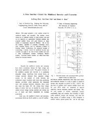
everything from metal alloys to fiberglass. The two primary corporations currently<br />
manufacturing such cables are 3M with its Aluminum Clad Composite Rein<strong>for</strong>ced<br />
(ACCR) conductor and CTC with its Aluminum Clad Composite Core (ACCC)<br />
conductor. These conductors are shown in Figures 1.4 and 1.5 respectively. Both <strong>of</strong><br />
<strong>the</strong>se cables use fully annealed aluminum wires on <strong>the</strong> outside that are supported by <strong>the</strong>se<br />
new composite core wires on <strong>the</strong> inside. What makes <strong>the</strong> composite cores special is <strong>the</strong>ir<br />
rate <strong>of</strong> <strong>the</strong>rmal expansion which is several times less than that <strong>of</strong> steel. Decreasing<br />
<strong>the</strong>rmal expansion is critical because on <strong>the</strong> majority <strong>of</strong> transmission lines <strong>the</strong> <strong>the</strong>rmal<br />
limit <strong>for</strong> that line is first reached, not when <strong>the</strong> temperature is great enough to cause <strong>the</strong><br />
steel to mechanically fail, but when <strong>the</strong> temperature is great enough to cause <strong>the</strong> steel to<br />
sag below regulated clearances.<br />
Figure 1.3. ACSR/TW<br />
8
Figure 1.4. 3M Aluminum Clad Composite Rein<strong>for</strong>ced<br />
Figure 1.5. CTC Aluminum Clad Composite Core<br />
9
One <strong>of</strong> <strong>the</strong> most exciting things about <strong>the</strong>se advanced conductors is <strong>the</strong> fact that<br />
identical diameter composite conductors can be hung in place <strong>of</strong> standard ACSR<br />
conductors. The composite conductors already in production require nearly <strong>the</strong> same<br />
amount <strong>of</strong> tension as <strong>the</strong>ir ACSR equivalent and could <strong>the</strong>re<strong>for</strong>e be strung on towers<br />
designed <strong>for</strong> a certain size ACSR conductor. This has <strong>the</strong> potential to allow utilities to be<br />
able to merely reconductor <strong>the</strong>ir existing transmission lines and greatly increase <strong>the</strong>ir<br />
transmission capacity.<br />
Composite conductors also allow <strong>for</strong> smaller sized conductors to achieve <strong>the</strong> same<br />
amount <strong>of</strong> ampacity as a larger ACSR conductor. Because <strong>the</strong> composite conductors are<br />
more heat resistant and <strong>the</strong>re<strong>for</strong>e can conduct more current than a normal ACSR<br />
conductor, if a utility wishes to build a new line with a specific ampacity a smaller<br />
composite conductor may be used. This is significant because smaller conductors require<br />
less tension when <strong>the</strong>y are strung, and this reduced tension translates into reduced tower<br />
size. Lowering <strong>the</strong> tower size not only reduces <strong>the</strong> capital spent on transmission towers,<br />
but potentially allows <strong>for</strong> smaller right <strong>of</strong> ways, which could greatly reduce <strong>the</strong> cost <strong>of</strong> a<br />
new transmission line to a utility.<br />
1.4 Thesis Outline<br />
The purpose <strong>of</strong> this <strong>the</strong>sis is to create a control method capable <strong>of</strong> running<br />
automated tests on advanced conductors. This control method will require calculating <strong>the</strong><br />
real time ampacity <strong>for</strong> a bare overhead conductor. The in<strong>for</strong>mation obtained from this<br />
10
will <strong>the</strong>n be used to control <strong>the</strong> current level running through <strong>the</strong> test lines so that <strong>the</strong>y<br />
can be maintained at specific temperatures <strong>for</strong> long periods <strong>of</strong> time.<br />
1.5 Chapter Outlines<br />
Chapter 2 is summary <strong>of</strong> capabilities <strong>of</strong> <strong>the</strong> PCAT test facility and some <strong>of</strong> <strong>the</strong> design<br />
considerations that went into its construction.<br />
Chapter 3 is a detailed discussion <strong>of</strong> <strong>the</strong> ampacity model developed to describe <strong>the</strong> real<br />
time behavior <strong>of</strong> <strong>the</strong> test lines.<br />
Chapter 4 discusses PCATamp, <strong>the</strong> program written to implement <strong>the</strong> ampacity model<br />
and control testing at <strong>the</strong> ORNL PCAT facility.<br />
Chapter5 discusses <strong>the</strong> results <strong>of</strong> using this control method to maintain a conductor at a<br />
specific temperature.<br />
Chapter 6 provides conclusions and recommendations <strong>for</strong> future work.<br />
11
Chapter 2<br />
POWERLINE CONDUCTOR ACCELERATED TEST FACILITY<br />
The control developed later on in this <strong>the</strong>sis was designed <strong>for</strong> use at Oak Ridge<br />
National Laboratory’s Powerline Conductor Accelerated Test (PCAT) Facility. The<br />
purpose <strong>of</strong> <strong>the</strong> PCAT facility is to allow <strong>the</strong> rapid testing and certification <strong>of</strong> new and<br />
advanced bare overhead transmission conductors. It is hoped that by per<strong>for</strong>ming <strong>the</strong>se<br />
tests, utilities will be encouraged to begin investing in some <strong>of</strong> <strong>the</strong>se new technologies<br />
that promise to help relieve some <strong>of</strong> <strong>the</strong> strain on <strong>the</strong> national transmission grid. The<br />
PCAT facility was one <strong>of</strong> <strong>the</strong> first parts <strong>of</strong> <strong>the</strong> Department <strong>of</strong> Energy’s (DOE) National<br />
Transmission Technology Research (NTTRC) initiative meant to promote research and<br />
development in transmission technology.<br />
This chapter will begin by giving an overview <strong>of</strong> <strong>the</strong> PCAT facility and how it<br />
typically operates. After that some <strong>of</strong> <strong>the</strong> design considerations that went into its<br />
construction will be discussed. The chapter will <strong>the</strong>n move on to a complete description<br />
<strong>of</strong> <strong>the</strong> many components that make up <strong>the</strong> facility and will wind up with a discussion <strong>of</strong><br />
<strong>the</strong> numerous measurement systems utilized.<br />
2.1 Overview<br />
The PCAT facility, pictured in Figure 2.1, allows <strong>the</strong> testing <strong>of</strong> a 2400ft section <strong>of</strong><br />
bare overhead conductor. This 2400ft section <strong>of</strong> conductor consists <strong>of</strong> two 1200ft<br />
sections <strong>of</strong> wire. These sections are strung on both sides <strong>of</strong> three high-voltage<br />
12
Figure 2.1. PCAT Site Photo<br />
transmission towers according to <strong>the</strong> IEEE Standard 524-2003 <strong>for</strong> installing overhead<br />
transmission line conductor. The facility is visualized in Figures 2.2 and 2.3. <strong>Conductors</strong><br />
strung at <strong>the</strong> test facility will <strong>the</strong>n typically undergo a number <strong>of</strong> rapid aging tests where<br />
<strong>the</strong> temperature <strong>of</strong> <strong>the</strong> conductor will be increased to 300°C. This rise in temperature is<br />
accomplished by running large currents through <strong>the</strong> line by connecting it to <strong>the</strong> positive<br />
and negative poles <strong>of</strong> a 2MW DC converter. The specifics <strong>of</strong> each test are determined on<br />
a case by case basis with each <strong>of</strong> <strong>the</strong> customers utilizing <strong>the</strong> test center. An array <strong>of</strong><br />
measuring devices are used throughout PCAT, from a complete wea<strong>the</strong>r station, to<br />
<strong>the</strong>rmocouples measuring actual conductor temperature, to readings <strong>of</strong> <strong>the</strong> voltage and<br />
current present on <strong>the</strong> line. All <strong>of</strong> this data is <strong>the</strong>n collected back at a measurement<br />
building, on site, <strong>for</strong> later analysis by ORNL and its customers.<br />
13
Figure 2.2. PCAT Side view Diagram<br />
Figure 2.3. PCAT Overhead Diagram<br />
14
2.2 Design<br />
Basic design elements were taken from a similar facility built at Georgia Power to<br />
validate ampacity models. The apparatus used by Georgia Power and Georgia Tech<br />
consisted <strong>of</strong> a 700ft section <strong>of</strong> 336 kcmil ACSR that could be energized with <strong>the</strong> use <strong>of</strong> a<br />
480V trans<strong>for</strong>mer [4]. Their setup also included a wea<strong>the</strong>r station, <strong>the</strong> use <strong>of</strong> ungrounded<br />
<strong>the</strong>rmocouples to measure actual conductor temperature, and <strong>the</strong> use <strong>of</strong> desktop<br />
computers to facilitate <strong>the</strong> data collection from all <strong>of</strong> <strong>the</strong>ir measurement devices [4].<br />
Many <strong>of</strong> <strong>the</strong>se elements would be carried over or taken into consideration during <strong>the</strong><br />
construction <strong>of</strong> PCAT.<br />
The differences that exist between <strong>the</strong> two facilities are primarily due to <strong>the</strong>ir<br />
different goals. Georgia Tech was interested in validating ampacity models. They<br />
needed to be able to load <strong>the</strong> line and to regulate it, but <strong>the</strong>y did not need to control <strong>the</strong><br />
current on <strong>the</strong> line in real time [4]. PCAT was designed to run tests on conductors that<br />
required fine control <strong>of</strong> <strong>the</strong> currents placed online to ei<strong>the</strong>r maintain a specified current or<br />
temperature. Utilizing auto-trans<strong>for</strong>mers at ORNL as <strong>the</strong>y did in Georgia simply could<br />
not satisfy this need. There<strong>for</strong>e <strong>the</strong> researchers at ORNL decided to use a DC power<br />
source instead <strong>of</strong> an AC power source. The o<strong>the</strong>r primary difference between <strong>the</strong> facility<br />
at Georgia Power and at ORNL is an issue <strong>of</strong> scale. Georgia Power’s apparatus used<br />
poles designed <strong>for</strong> distribution level systems to hang <strong>the</strong>ir lines [4]. Distribution poles<br />
were not tall enough, however, <strong>for</strong> <strong>the</strong> PCAT facility. Because <strong>the</strong> facility at ORNL was<br />
designed <strong>for</strong> high temperatures, it had to be able to maintain safe clearances <strong>for</strong> <strong>the</strong> sags<br />
15
produced by <strong>the</strong>se loads. Researchers at ORNL also wanted to be able to string a much<br />
larger section <strong>of</strong> conductor than was done in Georgia. The combined need to support <strong>the</strong><br />
increased strain <strong>of</strong> a larger conductor and maintain safe clearances from conductor sag,<br />
prompted ORNL to consult with <strong>the</strong> Tennessee Valley Authority (TVA) on <strong>the</strong> best way<br />
to proceed. They recommended <strong>the</strong> use <strong>of</strong> heavily guyed transmission grade towers.<br />
Specifically, three towers were used 600ft apart to allow two 1200ft sections <strong>of</strong> conductor<br />
to be strung on <strong>the</strong>m.<br />
The measurement requirements <strong>of</strong> both facilities were very similar and <strong>the</strong>re<strong>for</strong>e<br />
<strong>the</strong>ir setups <strong>for</strong> measurement are both similar. The two test centers were both interested<br />
in <strong>the</strong> conductor temperature, and <strong>the</strong> best way to acquire that temperature was to have<br />
<strong>the</strong>rmocouples on <strong>the</strong> line. PCAT chose to use ungrounded <strong>the</strong>rmocouples connected to a<br />
fiber optic network to ensure electric isolation between <strong>the</strong> line and <strong>the</strong> data collection<br />
computers. Both test centers are also outdoor facilities which created a need <strong>for</strong> wea<strong>the</strong>r<br />
stations.<br />
2.3 PCAT Facility Components<br />
A number <strong>of</strong> structures, equipment, and devices are necessary to operate <strong>the</strong><br />
Powerline Conductor Accelerated Test facility efficiently and safely. This section will<br />
attempt to detail many <strong>of</strong> <strong>the</strong> components used in this system, from <strong>the</strong> structures utilized,<br />
to <strong>the</strong> equipment required <strong>for</strong> each <strong>of</strong> <strong>the</strong> many measurements that are taken.<br />
16
2.4 Structures<br />
Six major structures make up <strong>the</strong> test site. There are two dead-end towers that<br />
consist <strong>of</strong> two 85ft steel poles and a midspan tower composed <strong>of</strong> a single 85ft steel pole.<br />
Then <strong>the</strong>re is a tractor trailor used to house <strong>the</strong> DC power supply and circuit breakers.<br />
Next to that is a mobile <strong>of</strong>fice building that houses <strong>the</strong> PCs and o<strong>the</strong>r equipment<br />
necessary to control <strong>the</strong> power supply and access all <strong>the</strong> measurement equipment. Finally<br />
<strong>the</strong>re is a fiberglass tower used to string a wire over <strong>the</strong> two buildings <strong>for</strong> lighting<br />
protection. These elements are identified in two pictures <strong>of</strong> <strong>the</strong> PCAT facility shown in<br />
Figures 2.4 and 2.5.<br />
Dead-end<br />
Suspension<br />
Dead-end<br />
Power Supply<br />
Measurement<br />
Trailer<br />
Fiberglass<br />
Pole<br />
Figure 2.4. Overhead view <strong>of</strong> PCAT<br />
17
Dead-end<br />
Suspension<br />
Dead-end<br />
Power Supply<br />
Fiberglass Pole<br />
Figure 2.5. View <strong>of</strong> PCAT<br />
18
2.5 Power Supply<br />
The heart <strong>of</strong> <strong>the</strong> PCAT power supply is a Transrex ISR 2294, a 2MW SCR-based<br />
DC converter. This unit allows accurate control <strong>of</strong> <strong>the</strong> voltage and current applied to any<br />
<strong>of</strong> <strong>the</strong> test lines. Power is supplied to this converter through a 4.16kV air-cooled<br />
trans<strong>for</strong>mer that is connected to a 13.8kV line that runs near <strong>the</strong> facility. Both circuit<br />
breakers and overload circuit protection are included <strong>for</strong> safety. Power is delivered from<br />
<strong>the</strong> DC converter to <strong>the</strong> test line through four paralleled sections <strong>of</strong> very large ACC<br />
conductor. This was done to ensure that <strong>the</strong> wire needed to put power on <strong>the</strong> test line<br />
would not in any way affect or bottleneck <strong>the</strong> test system. The ACC conductors are<br />
connected to large bus plates located on <strong>the</strong> dead-end tower closest to <strong>the</strong> power supply.<br />
Jumper cables composed <strong>of</strong> <strong>the</strong> conductor currently being tested are used to connect <strong>the</strong><br />
bus plates to <strong>the</strong> 2400ft section <strong>of</strong> line.<br />
2.6 Instrumentation<br />
The PCAT facility uses several different types <strong>of</strong> instrumentation to record what<br />
is occurring on a test line at any point in time. Measurements are recorded once every<br />
minute and stored onto PCs <strong>for</strong> later data analysis. This section will go through many <strong>of</strong><br />
<strong>the</strong> measurements taken at <strong>the</strong> PCAT facility and <strong>the</strong> equipment necessary to take those<br />
measurements.<br />
Conductor temperature is measured by 40-80 <strong>the</strong>rmocouples placed on or inside<br />
<strong>the</strong> line being tested. These ungrounded <strong>the</strong>rmocouples are placed along <strong>the</strong> length <strong>of</strong> <strong>the</strong><br />
entire line and its dead-ends and splices. Thermocouples are ei<strong>the</strong>r attached using special<br />
19
high temperature conductive tape made by 3M or by being placed inside <strong>of</strong> <strong>the</strong> conductor<br />
by bird caging it and <strong>the</strong>n allowing friction to hold it in place.<br />
Sag in <strong>the</strong> line, created by elevating its temperature, is measured directly by a<br />
laser centered between <strong>the</strong> mid-span tower and <strong>the</strong> dead-end tower nearest to <strong>the</strong> power<br />
supply. Sag may also be measured indirectly by two load cells connected to both sides <strong>of</strong><br />
<strong>the</strong> conductor, <strong>the</strong>se units also make it possible to constantly monitor <strong>the</strong> tension that <strong>the</strong><br />
line is under.<br />
A number <strong>of</strong> devices are used to also measure <strong>the</strong> wea<strong>the</strong>r conditions present at<br />
<strong>the</strong> test facility. The wea<strong>the</strong>r attributes recorded at <strong>the</strong> PCAT facility are listed below.<br />
• Ambient temperature (°C)<br />
• Solar radiation (watts per meters squared)<br />
• Wind speed (feet per second)<br />
• Wind direction (degrees)<br />
• Wind elevation (degrees)<br />
The majority <strong>of</strong> <strong>the</strong> measurement apparatuses used are connected to <strong>the</strong><br />
measurement trailer by an RS-485 network. The measurements are read by PC and<br />
logged to dated files every minute. These files are <strong>the</strong>n stored indefinitely so <strong>the</strong> data<br />
may be analyzed later as necessary. A single PC controls <strong>the</strong> power supply and<br />
measurement network. A second PC copies <strong>the</strong> online data files and runs a web server<br />
that allows <strong>for</strong> easy remote monitoring <strong>of</strong> <strong>the</strong> system.<br />
20
2.7 Summary<br />
The Power Line Conductor Accelerated Test facility is uniquely setup <strong>for</strong> <strong>the</strong><br />
testing <strong>of</strong> advanced overhead conductors. Its ability to precisely control very high current<br />
levels, while accurately measuring multiple line characteristics, makes it a one <strong>of</strong> a kind<br />
research facility. At <strong>the</strong> same time, <strong>the</strong> use <strong>of</strong> standard stringing equipment and<br />
transmission grade towers places test conductors in a setting similar to what <strong>the</strong>y would<br />
experience in <strong>the</strong> field. It is hoped that by providing <strong>the</strong>se capabilities PCAT will<br />
encourage utilities to adopt <strong>the</strong> conductors tested here earlier, providing <strong>the</strong>m with a way<br />
to cost effectively increase <strong>the</strong>ir transmission capacity.<br />
21
Chapter 3<br />
AMPACITY<br />
Calculating <strong>the</strong> current-temperature relationship <strong>of</strong> overhead conductors is not a<br />
new area <strong>of</strong> study. Over <strong>the</strong> years transient models have been developed that are capable<br />
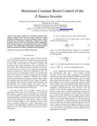
<strong>of</strong> calculating <strong>the</strong> temperature <strong>of</strong> an overhead conductor in real time. In 1993 IEEE<br />
released a revised version <strong>of</strong> <strong>the</strong>ir standard, 738, <strong>for</strong> calculating <strong>the</strong> current-temperature<br />
relationship <strong>of</strong> bare overhead conductors. That standard outlines <strong>the</strong> basic heat balance<br />
equation, discussed in detail later, first proposed by House and Tuttle [5]. The equation:<br />
dTc<br />
2<br />
qc + qr<br />
+ mCp<br />
= qs<br />
+ I ⋅ R(<br />
T<br />
dt<br />
broke up <strong>the</strong> energy balance into <strong>the</strong> heat created by conductive resistance, I 2 ·R, and <strong>the</strong><br />
heat absorbed from <strong>the</strong> sun, qs, with <strong>the</strong> heat lost to space and air through convection, qc,<br />
and radiation, qr. The transient equation also accounted <strong>for</strong> <strong>the</strong> heat storage <strong>of</strong> <strong>the</strong> line<br />
represented by<br />
mC<br />
p<br />
dT<br />
dt<br />
c<br />
. Over <strong>the</strong> years more and more accurate methods have been<br />
developed to calculate all <strong>the</strong>se different parts <strong>of</strong> <strong>the</strong> heat balance equation. Much <strong>of</strong> <strong>the</strong><br />
advancement in <strong>the</strong>se individual models has been made possible by <strong>the</strong> ability to solve<br />
<strong>the</strong>ir more complex ma<strong>the</strong>matical <strong>for</strong>ms with cheap computer power. Indeed, later in this<br />
chapter, a modified method is introduced <strong>for</strong> calculating <strong>the</strong> heat absorbed from <strong>the</strong> sun<br />
that is computationally taxing by even modern PC hardware.<br />
The first development <strong>of</strong> an ampacity model <strong>for</strong> bare overhead conductors was<br />
done by House and Tuttle in 1959. This was <strong>the</strong> first model to take into account <strong>the</strong><br />
22<br />
c<br />
)<br />
(3.1)
various <strong>for</strong>ces <strong>of</strong> wea<strong>the</strong>r that would affect <strong>the</strong> conductor. House and Tuttle also did <strong>the</strong><br />
first dissection <strong>of</strong> <strong>the</strong> heat balance equation into its various related parts, ie. heat loss<br />
through convection, and radiation and heat gain through solar radiation absorption and<br />
line losses because <strong>of</strong> impedance [6]. The field was largely left alone until <strong>the</strong> late<br />
1970’s when M. W. Davis wrote several articles on <strong>the</strong> subject <strong>of</strong> <strong>the</strong>rmal rating overhead<br />
lines.<br />
In 1982 Dr. W.Z. Black <strong>of</strong> Georgia Tech and many <strong>of</strong> his students began<br />
developing an ampacity model that would take advantage <strong>of</strong> new computing equipment.<br />
Dr. Black’s student, W.R. Byrd, wrote this first ampacity program <strong>for</strong> his Master’s Thesis<br />
[7]. This work was expanded by several more <strong>of</strong> Dr. Black’s students to take advantage<br />
<strong>of</strong> newer computers and better modeling techniques that maintained <strong>the</strong> model’s accuracy<br />
under high temperatures. PCATamp, <strong>the</strong> ampacity model that was developed <strong>for</strong> PCAT,<br />
was based largely on <strong>the</strong> work <strong>of</strong> Dr. W.Z. Black, W.R. Byrd, R.L. Rehberg, and S.L.<br />
Chen and could not have been done without <strong>the</strong>ir previous work [7,8,9].<br />
IEEE also created a standard in 1986, revised in 1993, <strong>for</strong> calculating <strong>the</strong> current-<br />
temperature relationship <strong>of</strong> bare overhead conductors. IEEE STD 738-1993 details a<br />
number <strong>of</strong> equations and algorithms that can be used to create an ampacity model.<br />
IEEE’s standard was also heavily referenced while creating PCATamp [5].<br />
3.1 <strong>Ampacity</strong> <strong>Model</strong><br />
In order to accurately control <strong>the</strong> PCAT facility, it was quickly realized that <strong>the</strong><br />
<strong>for</strong>ces at work on <strong>the</strong> conductor needed to be understood. Given <strong>the</strong> interest in<br />
23
controlling <strong>the</strong> temperature <strong>of</strong> <strong>the</strong> line by adjusting <strong>the</strong> current running through it, it made<br />
sense to develop a model <strong>of</strong> <strong>the</strong> current-temperature relationship, or ampacity, <strong>of</strong> <strong>the</strong><br />
conductors at <strong>the</strong> PCAT facility. Modern ampacity models account <strong>for</strong> not only <strong>the</strong> heat<br />
generated by conduction, but also <strong>the</strong> heat lost and gained due to <strong>the</strong> wea<strong>the</strong>r. Because <strong>of</strong><br />
<strong>the</strong> extensive measurement capabilities present at PCAT <strong>for</strong> everything from conductor<br />
temperature to solar radiation, it appeared that PCAT was in a prime position to utilize<br />
<strong>the</strong> body <strong>of</strong> work written on <strong>the</strong> ampacity <strong>of</strong> bare overhead conductors. The hundreds <strong>of</strong><br />
thousands <strong>of</strong> recorded data points at PCAT provided <strong>the</strong> in<strong>for</strong>mation necessary to build<br />
an accurate model that would most closely resemble what conductors experienced on a<br />
day-to-day basis.<br />
3.1.1 Heat Exchange<br />
The basic heat exchange equation <strong>for</strong> a bare overhead conductor is as follows [5,7]:<br />
where:<br />
dTc<br />
2<br />
qc + qr<br />
+ mCp<br />
= qs<br />
+ I ⋅ R(<br />
T<br />
dt<br />
q c = heat loss through convection (watts per linear foot <strong>of</strong> conductor)<br />
q r = heat loss through radiation (watts per linear foot <strong>of</strong> conductor)<br />
mC p = heat capacity <strong>of</strong> conductor (watt minutes per foot degrees centigrade)<br />
T c = conductor temperature (degrees centigrade)<br />
t = time (minutes)<br />
24<br />
c<br />
)<br />
(3.2)
q s = heat gain from <strong>the</strong> sun (watts per linear foot <strong>of</strong> conductor)<br />
I = conductor current (dc amps)<br />
R = resistance per linear foot <strong>of</strong> conductor at T c (ohms per foot)<br />
Rearranging this and solving <strong>the</strong> differential equation:<br />
2<br />
dTc I ⋅ R(<br />
Tc)<br />
+ qs<br />
− qc<br />
− q<br />
=<br />
dt<br />
mC<br />
makes it possible to calculate <strong>the</strong> conductor temperature at a specific time based on <strong>the</strong><br />
knowledge <strong>of</strong> each <strong>of</strong> <strong>the</strong> above conditions. An explanation <strong>of</strong> how this transient<br />
equation is solved will be provided later in this chapter.<br />
3.1.2 Qgen<br />
Qgen refers to <strong>the</strong> rate <strong>of</strong> heat generation in <strong>the</strong> line per unit length due to electrical<br />
2<br />
current. As part <strong>of</strong> <strong>the</strong> heat exchange equation, Qgen refers to R(<br />
Tc)<br />
25<br />
p<br />
r<br />
(3.3)<br />
I ⋅ . A great deal <strong>of</strong><br />
work has been done developing polynomial equations that accurately describe <strong>the</strong><br />
relationship between temperature and electrical impedance <strong>of</strong> a metal. However, at <strong>the</strong><br />
PCAT facility, solving a complex series <strong>of</strong> equations to describe <strong>the</strong> conductors overall<br />
impedance is unnecessary because <strong>the</strong> voltage and current on <strong>the</strong> line can be measured<br />
directly. This is desirable <strong>for</strong> a couple <strong>of</strong> reasons. Firstly, it reduces <strong>the</strong> amount <strong>of</strong><br />
calculation that needs to be done when <strong>the</strong> model is used in a real-time environment, and<br />
secondly it removes <strong>the</strong> dependence on accurately knowing <strong>the</strong> temperature-impedance<br />
relationship <strong>of</strong> a material. For typical conductor metals such as aluminum and steel, this
in<strong>for</strong>mation is well documented. However, part <strong>of</strong> PCAT’s design purpose is <strong>for</strong> <strong>the</strong><br />
testing <strong>of</strong> advanced overhead conductors, many <strong>of</strong> which are made out <strong>of</strong> new materials<br />
whose temperature-impedance relationship is ei<strong>the</strong>r unknown or undocumented in <strong>the</strong><br />
public sector.<br />
For PCATamp, Qgen is solved fairly directly. The resistance R is found by:<br />
where:<br />
V = measured voltage (dc volts)<br />
R =<br />
I = measured conductor current (dc amps)<br />
26<br />
V<br />
I<br />
2400<br />
Because R is in ohms per linear foot <strong>of</strong> conductor V I is divided by <strong>the</strong> length <strong>of</strong> <strong>the</strong><br />
conductor, 2400 feet.<br />
After <strong>the</strong> resistance is found, Qgen is calculated exactly like in <strong>the</strong> heat exchange<br />
equation. There is no need to worry about <strong>the</strong> temperature-resistance relationship<br />
because <strong>the</strong> resistance is being measured online.<br />
(3.4)<br />
It is worth noting that this method <strong>of</strong> calculating <strong>the</strong> heat produced by power<br />
losses is different from <strong>the</strong> bulk <strong>of</strong> <strong>the</strong> work per<strong>for</strong>med in ampacity modeling. This is<br />
because most ampacity models are set up to describe <strong>the</strong> power losses <strong>of</strong> an AC system,<br />
whereas PCAT uses a DC based power supply. The primary difference involves <strong>the</strong> fact<br />
that in an AC system skin-effect will increase <strong>the</strong> overall impedance <strong>of</strong> <strong>the</strong> line to some<br />
degree. In ampacity models designed <strong>for</strong> AC systems, this is accounted <strong>for</strong> in <strong>the</strong><br />
temperature-resistance curves that <strong>the</strong> system uses to track <strong>the</strong> overall resistivity <strong>of</strong> <strong>the</strong>
line. PCATamp does not account <strong>for</strong> things like skin-effect because it is a DC system<br />
and <strong>the</strong> facility is capable <strong>of</strong> directly measuring voltage and current online. Because<br />
PCAT is a DC system, readers should not assume current-temperature relationships <strong>for</strong> a<br />
specific line would apply in a utility setting under AC conditions. While <strong>the</strong>se<br />
relationships are used internally to control <strong>the</strong> behavior <strong>of</strong> <strong>the</strong> test facility, <strong>the</strong>y are not<br />
meant to describe <strong>the</strong> conductor under AC conditions. Cable manufacturers should be<br />
consulted <strong>for</strong> such in<strong>for</strong>mation.<br />
3.1.3 Mass Specific Heat Capacity<br />
The mass specific heat capacity, mCp, is an index <strong>of</strong> how well a material retains<br />
heat. While temperature dependent polynomials exist to describe <strong>the</strong> mass specific heat<br />
<strong>of</strong> normal conductors [7], 3M only provides singular average values <strong>for</strong> <strong>the</strong> materials in<br />
<strong>the</strong>ir advanced composite conductors. This is relevant, as all <strong>of</strong> <strong>the</strong> testing <strong>of</strong> PCATamp<br />
has been done on 3M’s novel ACCR conductor. 3M states that <strong>the</strong> mass specific heat <strong>for</strong><br />
<strong>the</strong> aluminum used in <strong>the</strong>ir conductor is 520 J/ft°C and 28 J/ft°C <strong>for</strong> <strong>the</strong>ir aluminum<br />
composite material. Because independent values are given <strong>for</strong> <strong>the</strong> mass specific heat, <strong>the</strong><br />
equation <strong>for</strong> mCp is simply:<br />
mC<br />
p<br />
mC<br />
=<br />
pAl<br />
27<br />
+ mC<br />
Division by 60 is necessary to convert J/ft°C to Watt Minutes/ft°C.<br />
60<br />
pCo<br />
(3.5)
3.1.4 Qcon<br />
The heat lost from a bare overhead conductor due to convection is built on a well<br />
developed method <strong>of</strong> determining convection heat losses by deriving <strong>the</strong> Grash<strong>of</strong>,<br />
Nusselt, and Reynolds numbers associated with <strong>the</strong> system [7,8]. Measured values <strong>of</strong><br />
wind speed and wind direction are used along with knowledge <strong>of</strong> <strong>the</strong> ambient<br />
temperature and conductor temperature to realize <strong>the</strong> rate at which heat will leave <strong>the</strong><br />
bare metal <strong>of</strong> <strong>the</strong> conductor <strong>for</strong> <strong>the</strong> air. This method <strong>of</strong> calculating <strong>the</strong> heat losses<br />
associated with convection was derived by Byrd and Rehberg in <strong>the</strong>ir <strong>the</strong>sis on ampacity<br />
[7,8]. The algorithm used to determine Qcon will be briefly discussed. For a more<br />
thorough explanation it is recommended that <strong>the</strong> reader consult those two <strong>the</strong>ses.<br />
Variables:<br />
wDir = measured wind direction (radians)<br />
wSpeed<br />
= measured wind speed (meters per second)<br />
Averages <strong>of</strong> <strong>the</strong>se two measurements are used due to <strong>the</strong> fairly noisy nature <strong>of</strong> wind<br />
measurement.<br />
D = diameter <strong>of</strong> <strong>the</strong> conductor (meters)<br />
Zl = line orientation <strong>of</strong> <strong>the</strong> conductor (radians)<br />
TC = conductor temperature (°C)<br />
TA = measured ambient temperature (°C)<br />
Pr = Prandtl Number (0.71)<br />
v = kinematic viscosity <strong>of</strong> air (m 2 /s)<br />
?wind = wind direction with respect to line orientation (radians)<br />
28
First <strong>the</strong> film temperature around <strong>the</strong> conductor will be found. This is <strong>the</strong> temperature <strong>of</strong><br />
<strong>the</strong> junction where <strong>the</strong> metal <strong>of</strong> <strong>the</strong> conductor meets <strong>the</strong> air. The conductor temperature<br />
is an average <strong>of</strong> 10 <strong>the</strong>rmocouples placed on and inside <strong>the</strong> test conductor. The ambient<br />
temperature is measured by <strong>the</strong>rmocouples hanging in <strong>the</strong> air <strong>of</strong>f <strong>of</strong> <strong>the</strong> tower closest to<br />
<strong>the</strong> power supply.<br />
T<br />
film<br />
T<br />
=<br />
Next determine <strong>the</strong> angle <strong>of</strong> <strong>the</strong> wind direction with respect to <strong>the</strong> line orientation by<br />
per<strong>for</strong>ming a cross product.<br />
θ<br />
Wind<br />
Next determine <strong>the</strong> air viscosity.<br />
C<br />
29<br />
+ T<br />
2<br />
= ArcSin (( Cos(<br />
Zl ) ⋅Sin(<br />
wDir<br />
)) − ( Cos(<br />
wDir<br />
) ⋅Sin(<br />
Zl<br />
)))<br />
π<br />
ω = −θ<br />
2<br />
wind<br />
2<br />
v f<br />
film<br />
film<br />
= ( 1.<br />
0167E<br />
−10⋅T<br />
+ 8.<br />
7305E<br />
−8<br />
⋅T<br />
+ 1.<br />
3888E<br />
−5<br />
Next determine <strong>the</strong> <strong>the</strong>rmal conductivity <strong>of</strong> <strong>the</strong> air.<br />
k<br />
f<br />
2<br />
= −2.<br />
7628E<br />
− 8⋅T<br />
film + 7.<br />
2316E<br />
− 5⋅T<br />
film +<br />
A<br />
0.<br />
023681<br />
Next calculate <strong>the</strong> product <strong>of</strong> <strong>the</strong> gravitational constant (g) and <strong>the</strong> coefficient <strong>of</strong> <strong>the</strong>rmal<br />
expansion <strong>for</strong> air (B) divided by <strong>the</strong> kinematic viscosity <strong>of</strong> air squared.<br />
(3.6)<br />
(3.7)<br />
(3.8)<br />
(3.9)<br />
(3.10)
g ⋅ B<br />
= 1.<br />
024E4<br />
⋅T<br />
2<br />
v<br />
Next determine <strong>the</strong> Grash<strong>of</strong> number.<br />
2<br />
film<br />
− 2.<br />
394E6<br />
⋅ T<br />
g ⋅ B 3<br />
Gr = ⋅ D ⋅ ( T<br />
2<br />
C − T<br />
v<br />
Next determine <strong>the</strong> Nusselt number <strong>for</strong> natural convection.<br />
x = log 10( Gr<br />
⋅ Pr<br />
)<br />
30<br />
A<br />
film<br />
)<br />
_1.<br />
85E8<br />
2<br />
ltNuNa = 0.<br />
12724 + ( 0.<br />
02238⋅<br />
x)<br />
+ ( 0.<br />
04203⋅<br />
x ) − ( 0.<br />
0025973⋅<br />
x<br />
Next find <strong>the</strong> Reynolds number.<br />
ltNuNa<br />
NuNa = 10<br />
R<br />
e<br />
=<br />
w<br />
Speed<br />
v<br />
f<br />
⋅ D<br />
Next find <strong>the</strong> Nusselt number <strong>for</strong> <strong>for</strong>ced convection.<br />
ltNuUc = −<br />
⋅<br />
0. 070431+<br />
0.<br />
31526 ⋅ log 10 ( Re<br />
) + 0.<br />
035527 log 10 ( Re<br />
ltNuUc<br />
NuUc = 10<br />
NuFc = NuUc⋅<br />
( 1.<br />
194 − Sin ( ω ) − ( 0.<br />
194 ⋅ Cos(<br />
2ω<br />
)) + ( 0.<br />
368 ⋅ Sin ( 2ω)))<br />
3<br />
)<br />
)<br />
2<br />
(3.11)<br />
(3.12)<br />
(3.13)<br />
(3.14)<br />
(3.15)<br />
(3.16)<br />
(3.17)<br />
(3.18)<br />
(3.19)
Next <strong>the</strong> convective heat transfer coefficients <strong>for</strong> natural and <strong>for</strong>ced convection will be<br />
found. A third coefficient corresponding to <strong>the</strong> average <strong>of</strong> <strong>the</strong> two will also be found to<br />
s<strong>of</strong>ten a potential discontinuity when solving <strong>the</strong> transient equation, discussed fur<strong>the</strong>r on<br />
<strong>the</strong> next page.<br />
Natural:<br />
Forced:<br />
Average:<br />
h<br />
Avg<br />
h<br />
h<br />
Na<br />
Fc<br />
NuNa⋅k<br />
=<br />
D<br />
NuFc ⋅ k<br />
=<br />
D<br />
NuNa + NuFc<br />
⋅ k<br />
= 2<br />
D<br />
Next <strong>the</strong> actual convective heat loss <strong>for</strong> each type <strong>of</strong> convection will be found. Division<br />
by 3.2808399 is per<strong>for</strong>med to convert watts per meter to watts per foot.<br />
Natural:<br />
Forced:<br />
Q<br />
conNa<br />
=<br />
h<br />
Na<br />
⋅π<br />
⋅ D⋅<br />
( TC<br />
−TA)<br />
3.2808399<br />
31<br />
f<br />
f<br />
f<br />
(3.20)<br />
(3.21)<br />
(3.22)<br />
(3.23)
Average:<br />
Q<br />
Q<br />
conFc<br />
conAvg<br />
=<br />
=<br />
h<br />
h<br />
Fc<br />
Avg<br />
⋅π<br />
⋅ D⋅<br />
( TC<br />
−TA)<br />
3.2808399<br />
⋅π<br />
⋅ D ⋅ ( TC<br />
−TA<br />
)<br />
3.2808399<br />
After <strong>the</strong> different values <strong>of</strong> convective heat loss have been calculated, <strong>the</strong> one<br />
that is chosen and used to determine <strong>the</strong> ampacity <strong>of</strong> <strong>the</strong> conductor must be determined.<br />
For wind speeds that are equal to zero, or too small to measure, <strong>the</strong> value <strong>for</strong> natural<br />
convection will be used. When <strong>the</strong>re is a large amount <strong>of</strong> wind indicated by (NuFc ><br />
NuNa), <strong>the</strong> Q value <strong>for</strong> <strong>for</strong>ced convection will be used. For low speed winds where <strong>the</strong><br />
Nusselt Number <strong>for</strong> natural convection is higher than <strong>the</strong> Nusselt number <strong>for</strong> <strong>for</strong>ced<br />
convection (NuNa > NuFc), <strong>the</strong> average <strong>of</strong> <strong>the</strong> convection values is used. This is done to<br />
prevent <strong>the</strong> transient equation from facing a steep discontinuity when wind speed travels<br />
to or from zero. While this aspect is important <strong>for</strong> a model to be able to run through a<br />
section <strong>of</strong> historic data, it does not apply to <strong>the</strong> control developed <strong>for</strong> <strong>the</strong> PCAT facility.<br />
This is because <strong>the</strong> control is interested in <strong>the</strong> future temperature <strong>of</strong> <strong>the</strong> conductor based<br />
on present conditions, <strong>the</strong>re<strong>for</strong>e only <strong>the</strong> present wind condition is provided to <strong>the</strong> model<br />
eliminating <strong>the</strong> need to protect against changing wind patterns.<br />
3.1.5 Qrad<br />
Determining <strong>the</strong> net radiation transfer between <strong>the</strong> environment and <strong>the</strong> conductor<br />
is much simpler than determining <strong>the</strong> heat loss due to convection. It is assumed that <strong>the</strong><br />
area around <strong>the</strong> cable can be simplified as a black iso<strong>the</strong>rmal environment. The heat loss<br />
32<br />
(3.24)<br />
(3.25)
due to radiation can <strong>the</strong>n be found as follows, as with <strong>the</strong> calculation <strong>of</strong> Qcon <strong>the</strong><br />
derivation <strong>of</strong> this algorithm can be found in Byrd’s <strong>the</strong>sis [7].<br />
Variables:<br />
D = diameter <strong>of</strong> <strong>the</strong> conductor (meters)<br />
TC = conductor temperature (°C)<br />
TA = measured ambient temperature (°C)<br />
σ = Stefan-Boltzman constant (5.67E-8)<br />
e = emmissivity (0.35)<br />
3.1.6 Qsun<br />
Q<br />
rad<br />
ε ⋅ D ⋅π<br />
⋅σ<br />
⋅(<br />
T<br />
=<br />
C<br />
+<br />
273.<br />
15)<br />
3.<br />
2808399<br />
33<br />
4<br />
− ( T<br />
A<br />
+<br />
273.<br />
15)<br />
Calculating <strong>the</strong> heat absorbed from <strong>the</strong> sun turns out to be one <strong>of</strong> <strong>the</strong> most<br />
rigorous calculations in an ampacity model. The reason <strong>for</strong> this is <strong>the</strong> need to calculate<br />
<strong>the</strong> azimuth and elevation <strong>for</strong> <strong>the</strong> sun at <strong>the</strong> precise time <strong>of</strong> interest. Traditionally <strong>the</strong>se<br />
calculations have been reduced to simple polynomials that mimic <strong>the</strong> basic course <strong>of</strong> <strong>the</strong><br />
sun throughout a day. This was done because accurate calculations <strong>of</strong> <strong>the</strong>se values<br />
involve a huge number <strong>of</strong> trigonometric equations that must be calculated to accurately<br />
model <strong>the</strong> movement <strong>of</strong> planets. Alone <strong>the</strong>se calculations pose no problem <strong>for</strong> modern<br />
computers; but, constantly running <strong>the</strong>se calculations in a real time application can tax<br />
even today’s fastest processors. Because it is possible to run <strong>the</strong>se calculations on current<br />
4<br />
(3.26)
equipment, however, an accurate planetary movement model has been incorporated into<br />
this model. A section <strong>of</strong> visual basic code written by Gregg Pelletier based on an<br />
algorithm created by <strong>the</strong> National Oceanic and Atmospheric Administration (NOAA) was<br />
used to find <strong>the</strong> azimuth and elevation <strong>of</strong> <strong>the</strong> sun; this algorithm can be seen in Appendix<br />
IV. The calculations per<strong>for</strong>med by this section <strong>of</strong> code were confirmed to match both <strong>the</strong><br />
web-based azimuth and elevation calculators used by <strong>the</strong> NOAA, and ano<strong>the</strong>r solar<br />
position algorithm written <strong>for</strong> <strong>the</strong> National Renewable Energy Laboratory (NREL). The<br />
development <strong>of</strong> <strong>the</strong> solar position algorithm is far too rigorous to discuss here and it is<br />
recommended that <strong>the</strong> reader consult NREL’s technical report on “Solar Position<br />
Algorithm <strong>for</strong> Solar Radiation Applications” by I. Reda and A. Andreas if he needs more<br />
in<strong>for</strong>mation [10].<br />
The second part <strong>of</strong> calculating <strong>the</strong> radiation absorption from <strong>the</strong> sun is knowing<br />
how much solar radiation is present on <strong>the</strong> line. In previous ampacity models this was<br />
<strong>of</strong>ten reduced to a table that gave an approximate value <strong>of</strong> <strong>the</strong> solar radiation based on no<br />
obstructions between <strong>the</strong> surface and <strong>the</strong> sun, and <strong>the</strong> time <strong>of</strong> year. Luckily, at PCAT<br />
<strong>the</strong>re is a solar radiation sensor that can measure <strong>the</strong> solar radiation present at <strong>the</strong> facility.<br />
This is very nice because traditionally <strong>the</strong>re has been no way to account <strong>for</strong> clouds, etc. in<br />
a model. Once <strong>the</strong> azimuth <strong>of</strong> <strong>the</strong> sun, <strong>the</strong> elevation <strong>of</strong> <strong>the</strong> sun, and <strong>the</strong> amount <strong>of</strong> solar<br />
radiation is known, <strong>the</strong> heat absorbed by <strong>the</strong> sun can be calculated as follows. These<br />
equations were taken from <strong>the</strong> IEEE’s Standard 738-1993 and Byrd’s <strong>the</strong>sis [5,7].<br />
Variables:<br />
D = diameter <strong>of</strong> <strong>the</strong> conductor (meters)<br />
34
Zl = line orientation <strong>of</strong> <strong>the</strong> conductor (radians)<br />
Zc = azimuth <strong>of</strong> <strong>the</strong> sun (degrees)<br />
Hc = elevation <strong>of</strong> <strong>the</strong> sun (degrees)<br />
a = solar absorptivity (0.35)<br />
lSun = measured solar radation (watts per meter squared)<br />
3.1.7 Solution<br />
⎡ ⎛π ⋅ Hc ⎞ ⎛π ⋅ ( Zc<br />
− Zl<br />
) ⎞⎤<br />
θ = ArcCos⎢Cos⎜<br />
⎟⋅<br />
Cos⎜<br />
⎟⎥<br />
⎣ ⎝ 180 ⎠ ⎝ 180 ⎠⎦<br />
Q<br />
sun<br />
lSun<br />
D<br />
= α ⋅<br />
⋅Sin<br />
( θ ) ⋅<br />
10.<br />
7639104 12<br />
Solving <strong>the</strong> heat balance equation requires quite a bit <strong>of</strong> computational ef<strong>for</strong>t. So,<br />
as was originally recommended by <strong>the</strong> authors <strong>of</strong> DynAmp, a runge-kutta routine was<br />
used to per<strong>for</strong>m this calculation [7]. Specifically, <strong>the</strong> Visual Basic version <strong>of</strong> PCATamp<br />
used a static step-size Runge-Kutta-Fehlberg 4-5 (RKF45) routine, available in Appendix<br />
I. This routine was written in Visual Basic, with great difficulty, based on algorithms<br />
written in Fortran and C by Watts and Shampine [11]. The Visual Basic routine was<br />
checked against solutions to some known differential equations as well as <strong>the</strong> Matlab<br />
version <strong>of</strong> PCATamp that utilized a built in RKF45 routine with step size control to<br />
verify its correct functioning.<br />
35<br />
(3.27)<br />
(3.28)
3.2 Transient vs Steady State<br />
The heat balance equation can be solved in two <strong>for</strong>ms. It can be simplified to<br />
steady state <strong>for</strong>m and solved easily <strong>for</strong> <strong>the</strong> current used to achieve a specific temperature;<br />
or it can solved in <strong>the</strong> transient <strong>for</strong>m <strong>for</strong> <strong>the</strong> temperature that would be associated with<br />
running at a specific current through <strong>the</strong> line. Using PCAT’s historic data, both solutions<br />
<strong>of</strong> <strong>the</strong> heat balance equation were compared. It was found that <strong>the</strong> steady state solution,<br />
which was significantly less costly computationally, did not provide <strong>the</strong> accuracy<br />
necessary to use it as a control <strong>for</strong> <strong>the</strong> PCAT system. It makes sense why it did not work<br />
because an outdoor test facility is anything but steady state. The transient method was<br />
also tested, and after being run against 247,680 historic data points was found to predict<br />
<strong>the</strong> actual temperature <strong>of</strong> <strong>the</strong> line quite accurately. The average difference between <strong>the</strong><br />
modeled temperature and <strong>the</strong> actual temperature was 5.2115ºC. Considering that testing<br />
is typically on <strong>the</strong> order <strong>of</strong> 240ºC, a 5ºC differential was considered more than<br />
acceptable.<br />
3.3 Summary<br />
Chapter three outlined PCATamp, an ampacity model developed <strong>for</strong> use at <strong>the</strong><br />
PCAT test facility. Utilizing <strong>the</strong> large body <strong>of</strong> previous research in calculating <strong>the</strong><br />
ampacity <strong>of</strong> an overhead conductor a model was created that could calculate <strong>the</strong> heat<br />
exchange parameters affecting <strong>the</strong> line. Specifically, models were created to handle <strong>the</strong><br />
heat generated by conduction, <strong>the</strong> heat absorbed by solar radiation, <strong>the</strong> heat lost to<br />
36
convection, and <strong>the</strong> heat lost to radiation. After <strong>the</strong> ampacity model was developed it<br />
was tested and found to per<strong>for</strong>m well over a wide range <strong>of</strong> historic data.<br />
37
Chapter 4<br />
PCATAMP<br />
The purpose <strong>of</strong> PCATamp was to provide a better control method <strong>for</strong> <strong>the</strong> PCAT<br />
facility <strong>for</strong> regulating <strong>the</strong> temperature <strong>of</strong> a test conductor. Managing <strong>the</strong> effects <strong>of</strong> <strong>the</strong><br />
wea<strong>the</strong>r on an outdoor facility has proven to be quite difficult. Previous attempts to<br />
control <strong>the</strong> temperature <strong>of</strong> a conductor consisted <strong>of</strong> attempts to maintain a specific<br />
impedance on <strong>the</strong> line. Wind and o<strong>the</strong>r factors, however, resulted in major fluctuations in<br />
<strong>the</strong> temperature on <strong>the</strong> line while using this control scheme. The goal <strong>of</strong> PCATamp was<br />
to account <strong>for</strong> <strong>the</strong>se exogeneoss conditions in <strong>the</strong> hope <strong>of</strong> creating a tighter control. In<br />
order to accomplish this task, <strong>the</strong> first item that was undertaken was <strong>the</strong> development <strong>of</strong><br />
an ampacity model that could accurately describe <strong>the</strong> temperature on <strong>the</strong> line based on <strong>the</strong><br />
real time measurement <strong>of</strong> its voltage, current, and multiple wea<strong>the</strong>r conditions.<br />
4.1 Matlab Test Version<br />
The first part <strong>of</strong> PCATamp was <strong>the</strong> development <strong>of</strong> <strong>the</strong> ma<strong>the</strong>matical ampacity<br />
model which was built in Matlab. Utilizing <strong>the</strong> body <strong>of</strong> work on ampacity models<br />
discussed in <strong>the</strong> previous chapter, a program was written to solve <strong>for</strong> <strong>the</strong> temperature <strong>of</strong> a<br />
test conductor. This program was <strong>the</strong>n systematically run through some 247,680<br />
archived data points calculating <strong>the</strong> modeled temperature <strong>of</strong> one <strong>of</strong> <strong>the</strong> lines every minute<br />
<strong>for</strong> a four month period. The final result <strong>of</strong> this test version <strong>of</strong> <strong>the</strong> code had an average<br />
error <strong>of</strong> +/- 5º C from <strong>the</strong> actual recorded line temperature.<br />
38
Of note in <strong>the</strong> Matlab version <strong>of</strong> PCATamp are some <strong>of</strong> <strong>the</strong> decisions <strong>for</strong><br />
averaging that were made early on. First, <strong>the</strong> PCAT test facility is not only outdoor, but<br />
quite long. These attributes lead to differences in <strong>the</strong> measured temperatures along <strong>the</strong><br />
line. In fact differences between <strong>the</strong>rmocouples measuring line temperature have varied<br />
up to 15ºC due to varying wind conditions along <strong>the</strong> line. In light <strong>of</strong> <strong>the</strong>se variations it<br />
was decided that an average <strong>of</strong> 10 <strong>the</strong>rmocouples evenly spaced along <strong>the</strong> line would be<br />
recorded. It was determined that this average did <strong>the</strong> best job <strong>of</strong> describing <strong>the</strong><br />
temperature <strong>of</strong> <strong>the</strong> line overall and would be <strong>the</strong> most logical temperature to attempt to<br />
match with <strong>the</strong> ampacity model. Second, measuring <strong>the</strong> speed and direction <strong>of</strong> <strong>the</strong> wind<br />
tends to be a particularly noisy business. In order to smooth out <strong>the</strong> wind data, averages<br />
were taken. The length <strong>of</strong> time averaged was reduced as small as possible to attempt to<br />
ensure that while noise was reduced, wind gusts were not smoo<strong>the</strong>d out. This is<br />
important because gusts <strong>of</strong> wind can affect <strong>the</strong> temperature <strong>of</strong> <strong>the</strong> line by several degrees.<br />
4.2 Visual Basic Implementation<br />
After <strong>the</strong> ampacity model was built and verified in Matlab, it was decided that it<br />
was worth attempting to integrate <strong>the</strong> model into a control <strong>for</strong> <strong>the</strong> PCAT facility. All <strong>of</strong><br />
<strong>the</strong> existing control and monitoring s<strong>of</strong>tware had been written in Micros<strong>of</strong>t Visual Basic<br />
6.0, so it was decided that <strong>the</strong> easiest way to implement <strong>the</strong> model would be to simply<br />
rewrite it in Visual Basic as well.<br />
39
4.2.1 Implementing an ODE<br />
The first problem that was identified with writing a Visual Basic implementation<br />
was <strong>the</strong> loss <strong>of</strong> Matlab’s Ordinary Differential Equation solvers, specifically ODE45.<br />
ODE45 was used to calculate <strong>the</strong> transient heat balance equation in <strong>the</strong> Matlab version.<br />
Searching <strong>the</strong> internet quickly proved that not many people had previously considered<br />
using Visual Basic to solve a complex differential equation. In fact no existing Visual<br />
Basic code could be found that was capable <strong>of</strong> solving <strong>the</strong> ampacity model’s transient<br />
equation. Previous authors and indeed Matlab’s own ODE solvers used a Runge-Kutta-<br />
Fehlberg algorithm, so it was decided to simply attempt to implement such an algorithm<br />
in Visual Basic. Several versions <strong>of</strong> <strong>the</strong> Runge-Kutta-Fehlberg method exist written in<br />
Fortran and C. It was decided that <strong>the</strong> best version to implement was probably <strong>the</strong> very<br />
robust and straight <strong>for</strong>ward algorithm RKF45 initially developed by Watts and Shampine<br />
[11]. This algorithm uses a static stepsize Runge-Kutta-Fehlberg 4-5 th order method.<br />
While RKF45 is slightly less sophisticated than Matlab’s dynamic step size version, it<br />
could be implemented in Visual Basic and proved capable <strong>of</strong> solving <strong>the</strong> transient<br />
equation within several decimal places <strong>of</strong> <strong>the</strong> solutions calculated by Matlab. The Visual<br />
Basic version <strong>of</strong> RKF45 can be referenced in Appendix I.<br />
4.2.2 Implementing <strong>the</strong> <strong>Ampacity</strong> <strong>Model</strong><br />
After <strong>the</strong> problem <strong>of</strong> solving <strong>the</strong> transient equation had been solved, <strong>the</strong> rest <strong>of</strong><br />
conversion <strong>of</strong> <strong>the</strong> ampacity model was fairly straight<strong>for</strong>ward. The ampacity model<br />
implemented in Visual Basic is a nearly direct translation <strong>of</strong> <strong>the</strong> model described in<br />
Chapter 3 <strong>of</strong> this <strong>the</strong>sis, and can be seen in Appendix II. The only general issues that<br />
40
were encountered while writing <strong>the</strong> Visual Basic version <strong>of</strong> <strong>the</strong> ampacity model was <strong>the</strong><br />
lack <strong>of</strong> many advanced math functions in Visual Basic’s IDE. A module <strong>of</strong> necessary<br />
math functions had to be written and is included in this <strong>the</strong>sis in Appendix III.<br />
Some new code had to be created <strong>for</strong> calculating <strong>the</strong> azimuth and elevation <strong>of</strong><br />
<strong>the</strong> sun. The Matlab version <strong>of</strong> PCATamp previously used a section <strong>of</strong> code that<br />
implemented I. Reda and A. Andreas’s algorithm developed <strong>for</strong> <strong>the</strong> National Renewable<br />
Energy Laboratory (NREL) [10]. Instead <strong>of</strong> converting this large section <strong>of</strong> code over to<br />
Visual Basic, a Visual Basic version <strong>of</strong> a similar algorithm developed <strong>for</strong> <strong>the</strong> National<br />
Oceanic and Atmospheric Administration (NOAA) and translated to Visual Basic by G.<br />
Pelletier, was used. Both <strong>of</strong> <strong>the</strong>se algorithms were written to calculate <strong>the</strong> position <strong>of</strong> <strong>the</strong><br />
sun with extremely high accuracy and produce identical results. During debugging and<br />
optimization <strong>of</strong> PCATamp, <strong>the</strong> author realized how heavy a load calculating <strong>the</strong> location<br />
<strong>of</strong> <strong>the</strong> sun, in near real time, actually is. In fact some 90% <strong>of</strong> execution time would<br />
normally be spent inside <strong>of</strong> <strong>the</strong> sun module. In order to speed up PCATamp some<br />
modifications <strong>of</strong> <strong>the</strong> original sun code were made, at <strong>the</strong> expense <strong>of</strong> readability, in an<br />
ef<strong>for</strong>t to minimize process overhead. The code used <strong>for</strong> calculating <strong>the</strong> azimuth and<br />
elevation <strong>of</strong> <strong>the</strong> sun is located in Appendix IV.<br />
The only safety nets placed inside <strong>the</strong> ampacity model part <strong>of</strong> <strong>the</strong> PCATamp<br />
program is a program stop if <strong>the</strong> conductor temperature is below <strong>the</strong> ambient temperature.<br />
This condition will cause illegal ma<strong>the</strong>matical operations to occur and must <strong>the</strong>re<strong>for</strong>e be<br />
prevented. No o<strong>the</strong>r program stops have been coded due to <strong>the</strong> general resistance <strong>of</strong> <strong>the</strong><br />
algorithm to corruption, and its ability to handle very poor data. PCATamp was run<br />
continuously <strong>for</strong> several days with random input data to insure that odd data patterns<br />
41
would not cause <strong>the</strong> program to fail. Insuring that PCATamp would not crash erratically<br />
or get caught in situations <strong>of</strong> non-convergence was important because <strong>of</strong> <strong>the</strong> potential <strong>for</strong><br />
serious equipment damage.<br />
Even though PCATamp is quite resilient to crashing, however, it can not be run<br />
under extreme wea<strong>the</strong>r conditions. The ampacity model used is not capable <strong>of</strong><br />
accounting <strong>for</strong> <strong>the</strong> cooling effects <strong>of</strong> rain, or ice on <strong>the</strong> line. Because <strong>the</strong> effects <strong>of</strong> <strong>the</strong>se<br />
wea<strong>the</strong>r events can not be accounted <strong>for</strong> <strong>the</strong> ampacity model can not be counted on to<br />
provide a reliable answer. There<strong>for</strong>e operators must be aware <strong>of</strong> <strong>the</strong> prevailing wea<strong>the</strong>r<br />
conditions to know if suitable conditions exist <strong>for</strong> running PCATamp.<br />
4.3 Control Scheme<br />
The control created with PCATamp begins by taking data from <strong>the</strong> online<br />
instrumentation, including current, voltage, and wea<strong>the</strong>r conditions, and passing it to<br />
function PredictTempC, as seen in Appendix II. This function returns <strong>the</strong> expected<br />
temperature <strong>of</strong> <strong>the</strong> line at some time in <strong>the</strong> future, based on <strong>the</strong> present wea<strong>the</strong>r<br />
conditions and maintaining <strong>the</strong> present current value. The expected temperature is <strong>the</strong>n<br />
compared against a desired temperature <strong>for</strong> <strong>the</strong> line. If <strong>the</strong> expected temperature varies<br />
more than two degrees from <strong>the</strong> desired temperature, <strong>the</strong> current value in memory will be<br />
raised or lowered two amps and PredictTempC will be rerun. This process will continue<br />
until <strong>the</strong> expected and desired temperatures match. At that point, if <strong>the</strong> current value in<br />
memory has changed from <strong>the</strong> current value being commanded to <strong>the</strong> line, <strong>the</strong> new<br />
42
current value will be commanded to <strong>the</strong> system. PCATamp will <strong>the</strong>n wait one minute<br />
and start over. This process is illustrated in Figure 4.1 on <strong>the</strong> next page.<br />
For safety, PCATamp is not allowed to command large changes in <strong>the</strong> current.<br />
The control system will only allow <strong>the</strong> current change to be less than 300 amps per<br />
minute. This was done to prevent large steps in current that could cause damage to <strong>the</strong><br />
equipment on site. If PCATamp recommends a change <strong>of</strong> more than 300 amps <strong>the</strong><br />
system will change a maximum <strong>of</strong> 300 amps per minute, until <strong>the</strong> recommended change<br />
has been met. A check is also done to ensure that <strong>the</strong> actual temperature is not too far<br />
from <strong>the</strong> desired temperature, and if it is, <strong>the</strong> program shuts down. This could potentially<br />
happen if some un-modeled wea<strong>the</strong>r event is present on <strong>the</strong> line, such as rain. In this<br />
case, <strong>the</strong> line would be cooling far more than <strong>the</strong> ampacity model would be aware <strong>of</strong><br />
causing a disparity in temperatures.<br />
4.4 Summary<br />
Chapter four developed <strong>the</strong> Visual Basic control in use at PCAT <strong>for</strong> maintaining<br />
test conductors at a specific temperature. A number <strong>of</strong> challenges were discussed in<br />
converting <strong>the</strong> ampacity model from Matlab to Visual Basic. These challenges primarily<br />
involved <strong>the</strong> loss <strong>of</strong> <strong>the</strong> ordinary differential equation solvers built into Matlab. Next, <strong>the</strong><br />
control scheme used to maintain a test conductor at a specific temperature is discussed.<br />
The method used makes use <strong>of</strong> <strong>the</strong> ampacity model’s ability to predict <strong>the</strong> future<br />
temperature <strong>of</strong> <strong>the</strong> line and <strong>the</strong>n adjust <strong>the</strong> current level to drive <strong>the</strong> conductor<br />
temperature towards its target.<br />
43
Measure<br />
Wea<strong>the</strong>r<br />
Predict Future<br />
Temperature<br />
Measure<br />
Voltage<br />
Is <strong>the</strong> Yes<br />
predicted<br />
temperature<br />
acceptable? No<br />
Desired<br />
Temperature<br />
44<br />
Measure<br />
Current<br />
Command<br />
Current Variable<br />
Current<br />
Variable<br />
Adjust Current Variable<br />
And<br />
Repeat Control<br />
Figure 4.1. PCATamp Control Algorithm
Chapter 5<br />
EXPERIMENTAL RESULTS<br />
In <strong>the</strong> previous chapters, an ampacity model and a subsequent control based on<br />
that model were introduced. This chapter will take <strong>the</strong> developed control and discuss its<br />
per<strong>for</strong>mance online at <strong>the</strong> test facility. A number <strong>of</strong> factors were found to have<br />
significant effects on <strong>the</strong> per<strong>for</strong>mance <strong>of</strong> <strong>the</strong> control while tuning it online. Eventually it<br />
was discovered that variable sensitivity could be greatly altered by modifying <strong>the</strong> time<br />
constant that <strong>the</strong> control was using. This realization would result in a significant<br />
improvement in <strong>the</strong> per<strong>for</strong>mance <strong>of</strong> <strong>the</strong> control.<br />
5.1 Apparatus Setup<br />
The conductor being tested is 795 kcmil 3M ACCR. This composite cable is<br />
capable <strong>of</strong> temperatures up to 240°C. The conductor has <strong>the</strong> following specifications that<br />
apply to <strong>the</strong> control.<br />
• Number <strong>of</strong> Aluminum Strands = 26<br />
• Number <strong>of</strong> Composite Strands = 19<br />
• Diameter <strong>of</strong> Aluminum Wire = 0.175 in<br />
• Diameter <strong>of</strong> Composite Wire = 0.082 in<br />
• Diameter <strong>of</strong> Whole Conductor = 1.11 in<br />
• Heat Capacity <strong>of</strong> Aluminum = 324 J/ft°C<br />
• Heat Capacity <strong>of</strong> Composite = 22 J/ft°C<br />
45
It should be noted that this is not <strong>the</strong> conductor used to build and tune <strong>the</strong> initial<br />
ampacity model. The cable used <strong>for</strong> creating <strong>the</strong> model was a 1272 kcmil 3M ACCR<br />
conductor. The primary difference was that <strong>the</strong> previous conductor was significantly<br />
larger, with increased surface area, and increased heat capacities. However, <strong>the</strong> original<br />
model was setup with variables in place that could be modified accordingly per <strong>the</strong><br />
conductor that was being used. Setting <strong>the</strong> control up <strong>for</strong> online use with a different<br />
conductor posed some uncertainty because while <strong>the</strong> original model was setup to be<br />
capable <strong>of</strong> potentially handling any conductor, <strong>the</strong> effects <strong>of</strong> changing <strong>the</strong> conductor were<br />
at <strong>the</strong> time unknown. In <strong>the</strong> end, however, it was seen that <strong>the</strong> model behaved as it was<br />
designed.<br />
Measuring <strong>the</strong> conductor temperature is accomplished by using <strong>the</strong> average <strong>of</strong> 10<br />
<strong>the</strong>rmocouples along <strong>the</strong> line. These <strong>the</strong>rmocouples are evenly spaced approximately 150<br />
feet apart from each o<strong>the</strong>r along both sides <strong>of</strong> <strong>the</strong> conductor loop. The <strong>the</strong>rmocouples<br />
used are a combination <strong>of</strong> ones attached to <strong>the</strong> surface <strong>of</strong> <strong>the</strong> conductor and some that are<br />
imbedded next to <strong>the</strong> core <strong>of</strong> <strong>the</strong> conductor. All <strong>the</strong>rmocouple readings are per<strong>for</strong>med by<br />
ICP-DAS I-7018 <strong>the</strong>rmocouples, using type T <strong>the</strong>rmocouples. These units were all<br />
calibrated by hand using a high accuracy <strong>the</strong>rmocouple calibration device to within +/-<br />
0.1°C. A recent lightening strike that damaged several <strong>of</strong> <strong>the</strong> <strong>the</strong>rmocouples, resulting in<br />
<strong>the</strong>ir replacement, has insured that <strong>the</strong> <strong>the</strong>rmocouples now in place should be operating to<br />
<strong>the</strong> highest possible degree <strong>of</strong> accuracy.<br />
Wind speed and direction is measured by multiple devices in both two-<br />
dimensions and three-dimensions. For use with <strong>the</strong> control <strong>the</strong> data passed by <strong>the</strong> two<br />
dimensional measurement apparatus is used.<br />
46
Ambient temperature is measured by <strong>the</strong> same type <strong>of</strong> <strong>the</strong>rmocouples that are<br />
used to measure conductor temperature. Ambient temperature is measured by<br />
<strong>the</strong>rmocouples high on <strong>the</strong> tower placed out in <strong>the</strong> air.<br />
Solar radiation is measured by a solar radiation device capable <strong>of</strong> measuring watts<br />
per meter squared <strong>of</strong> solar radiation. Because this device is used in calculating <strong>the</strong> effect<br />
<strong>of</strong> solar radiation on <strong>the</strong> line <strong>the</strong> effects <strong>of</strong> cloud shading are taken into account as <strong>the</strong>y<br />
will be read as reduced exposure to solar radiation.<br />
5.2 Program Setup<br />
Program setup was relatively easy. The main modification made to <strong>the</strong> original<br />
PCAT control s<strong>of</strong>tware was <strong>the</strong> addition <strong>of</strong> a box, Figure 5.1, containing <strong>the</strong> available<br />
variables that could be modified <strong>for</strong> tuning <strong>the</strong> control. These variables included <strong>the</strong><br />
following.<br />
Time Stop: Time Stop was <strong>the</strong> variable used to control how far into <strong>the</strong> future<br />
<strong>the</strong> ampacity model would look. The variable effectively modified how many minutes<br />
PCATamp would model. For example, a Time Stop value <strong>of</strong> five indicated that<br />
PCATamp should output <strong>the</strong> expected temperature, based on present wea<strong>the</strong>r conditions,<br />
five minutes into <strong>the</strong> future. Typical values: 1 – 20 (integer)<br />
47
Figure 5.1. Temperature Tracking Box<br />
48
Update: This was <strong>the</strong> variable used to control how <strong>of</strong>ten a new current value<br />
could be commanded to <strong>the</strong> system. The original s<strong>of</strong>tware <strong>for</strong> PCAT operates on a<br />
watchdog clock <strong>of</strong> one minute that precisely dictates when to collect data from <strong>the</strong><br />
measurement devices and when to command <strong>the</strong> system to a different current value. The<br />
variable Update makes it possible to change how <strong>of</strong>ten <strong>the</strong> ampacity model could update<br />
<strong>the</strong> current on <strong>the</strong> system. For example, an Update value <strong>of</strong> one indicated that every<br />
minute <strong>the</strong> latest output <strong>of</strong> <strong>the</strong> control would be commanded to <strong>the</strong> system. An Update<br />
value <strong>of</strong> five would indicate that <strong>the</strong> control s<strong>of</strong>tware could only change <strong>the</strong> commanded<br />
current once every five minutes. This variable was introduced because <strong>of</strong> some initial<br />
concern that allowing <strong>the</strong> control to command <strong>the</strong> current every minute might lead to<br />
excessive switching <strong>for</strong> <strong>the</strong> power supply. Typical values: 1 – 5 (integer)<br />
Target Delta: This variable controlled how close to <strong>the</strong> target temperature <strong>the</strong><br />
control had to be. The PCATamp control returns a temperature based on present wea<strong>the</strong>r<br />
conditions and <strong>the</strong> current on <strong>the</strong> line. Modifying <strong>the</strong> target delta changes how near to<br />
that target temperature <strong>the</strong> control has to be to return an acceptable value <strong>for</strong><br />
commanding <strong>the</strong> current. For example, a target delta <strong>of</strong> five indicates that PCATamp has<br />
to provide a current value back to <strong>the</strong> control that results in an expected temperature that<br />
is +/-5°C <strong>of</strong> <strong>the</strong> temperature <strong>the</strong> control is attempting to hold <strong>the</strong> line at. Typical values:<br />
1 - 5 (float)<br />
Emissivity: Emissivity generally describes <strong>the</strong> condition <strong>of</strong> <strong>the</strong> air next to <strong>the</strong><br />
conductor. This value is modified based on attributes such as, is <strong>the</strong> line being tested on<br />
49
a mountain with clean air, or is it running through a major city with significant levels <strong>of</strong><br />
pollution in <strong>the</strong> air. The value <strong>for</strong> emmisivity was tuned during <strong>the</strong> development <strong>of</strong> <strong>the</strong><br />
model and should generally not require modification. However, should <strong>the</strong> model drift<br />
<strong>of</strong>f <strong>of</strong> <strong>the</strong> target temperatures during seasonal changes this variable can be used to<br />
account <strong>for</strong> such movement. Typical values: 0.23 - 0.91 (float)<br />
Current / Voltage: This variable is used to control how many current and<br />
voltage measurements are averaged toge<strong>the</strong>r <strong>for</strong> use with <strong>the</strong> control. A value <strong>of</strong> one here<br />
would indicate that <strong>the</strong> control is using real-time current and voltage data from line<br />
measurements. A value <strong>of</strong> five here would indicate that a moving average <strong>of</strong> five<br />
minutes <strong>of</strong> current values and voltage values would be passed to <strong>the</strong> control. The<br />
variable is present to account <strong>for</strong> <strong>the</strong> power supply’s inability to immediately change to<br />
specific commanded currents. For example, if a current <strong>of</strong> 1000 Amps is present online<br />
and a current <strong>of</strong> 1200 Amps is commanded to <strong>the</strong> line <strong>the</strong> power supply might first<br />
change to 1290 Amps and <strong>the</strong>n 1170 Amps and <strong>the</strong>n settle very close to <strong>the</strong> desired<br />
current value, all within a few seconds. This average allows this behavior to be smoo<strong>the</strong>d<br />
out <strong>for</strong> <strong>the</strong> control. Typical values: 1 – 3 (integer)<br />
Conductor / Ambient Temperature: This variable is used to control how many<br />
conductor temperature and ambient temperature values are averaged toge<strong>the</strong>r <strong>for</strong> use with<br />
<strong>the</strong> control. A value <strong>of</strong> one here would indicate that <strong>the</strong> control is using real-time<br />
temperature data <strong>of</strong>f <strong>the</strong> line. A value <strong>of</strong> five here would indicate that a moving average<br />
<strong>of</strong> five minutes <strong>of</strong> temperature data would be passed to <strong>the</strong> control. This variable is<br />
50
present because <strong>the</strong> reading from <strong>the</strong> <strong>the</strong>rmocouples are never constant and always float<br />
around based on <strong>the</strong> conditions present. The average is in place to smooth out <strong>the</strong>se<br />
values <strong>for</strong> a more consistent input to <strong>the</strong> control. Typical values: 1 – 3 (integer)<br />
Wind Speed / Wind Direction: This variable is used to control how many wind<br />
speed and wind direction measurements are averaged toge<strong>the</strong>r <strong>for</strong> use with <strong>the</strong> control.<br />
This variable is quite important because <strong>of</strong> <strong>the</strong> very noisy nature <strong>of</strong> both <strong>the</strong> wind speed<br />
and wind direction measurements. Because wind speed and wind direction are so noisy,<br />
an average <strong>of</strong> <strong>the</strong>ir values has to be per<strong>for</strong>med in order to have any indication <strong>of</strong> what <strong>the</strong><br />
overall wind pattern present is. Although <strong>the</strong> wind speed and wind direction variable is<br />
noisy, it is <strong>the</strong> most significant wea<strong>the</strong>r variable affecting <strong>the</strong> ampacity model. This<br />
makes finding <strong>the</strong> average value that provides enough real-time data but does not provide<br />
erratic data both difficult and very important. For example, a value <strong>of</strong> 45 here would<br />
indicate that a moving average <strong>of</strong> 45 minutes <strong>of</strong> wind speed and wind direction data<br />
would be passed to <strong>the</strong> control. Typical values: 5 – 45 (integer)<br />
Solar: This variable controls how many solar radiation values are averaged<br />
toge<strong>the</strong>r be<strong>for</strong>e being provided to <strong>the</strong> control. It operates very similarly to <strong>the</strong> variables<br />
mentioned above. For example, a value <strong>for</strong> five here would indicate that a five minute<br />
moving average <strong>of</strong> <strong>the</strong> solar radiation data is provided to <strong>the</strong> control. This variable is<br />
present to smooth any noise that may be present in <strong>the</strong> measurement. Typical values: 1 –<br />
5 (integer)<br />
51
Target Temperature: This is <strong>the</strong> target variable <strong>of</strong> <strong>the</strong> control. This variable<br />
sets what temperature <strong>the</strong> control should attempt to keep <strong>the</strong> temperature at. For<br />
example, a value <strong>of</strong> 190 would indicate that PCATamp should attempt to elevate and<br />
maintain <strong>the</strong> temperature <strong>of</strong> <strong>the</strong> conductor at 190°C. Typical values: 100 - 240 (integer)<br />
5.3 Control Tuning<br />
Tuning <strong>the</strong> control turned out somewhat unexpectedly. One <strong>of</strong> <strong>the</strong> initial<br />
configurations tested was as follows.<br />
• Time Stop = 10<br />
• Update = 5<br />
• Target Delta = 5<br />
• Emissivity = 0.35<br />
• Current / Voltage = 3<br />
• Conductor / Ambient Temperature = 3<br />
• Wind Speed / Direction = 45<br />
• Solar = 5<br />
• Target Temp = 100<br />
Figures 5.2 through 5.8 display graphs associated with this test. This test was run<br />
from 6:57pm on October 26, 2005 to 3:10pm on October 27, 2005. As can be seen from<br />
Figure 5.2, <strong>the</strong> conductor temperature remained slightly below <strong>the</strong> target <strong>of</strong> 100°C during<br />
<strong>the</strong> night, but during <strong>the</strong> day <strong>the</strong> control kept <strong>the</strong> temperature some 20°C above <strong>the</strong> target.<br />
It was discovered that <strong>the</strong>se variations were caused by a number <strong>of</strong> reasons.<br />
52
Conductor Temperature, °C<br />
140<br />
120<br />
100<br />
80<br />
60<br />
40<br />
20<br />
0<br />
Conductor Temperature - October 26,27 2005 (Target = 100°C)<br />
18:57:00 21:27:00 23:57:00 2:27:00 4:57:00 7:27:00 9:57:00 12:27:00 14:57:00<br />
Figure 5.2. Conductor Temperature – 10/26/2005 (Constant Temperature Test)<br />
Current, Amps<br />
1600<br />
1400<br />
1200<br />
1000<br />
800<br />
600<br />
400<br />
200<br />
53<br />
Time<br />
Current - October 26,27 2005 (Target = 100°C)<br />
0<br />
18:57:00 21:27:00 23:57:00 2:27:00 4:57:00 7:27:00 9:57:00 12:27:00 14:57:00<br />
Figure 5.3. Current – 10/26/2005 (Constant Temperature Test)<br />
Time
Wind Speed, ft/s<br />
Wind Azimuth, Degrees<br />
8<br />
7<br />
6<br />
5<br />
4<br />
3<br />
2<br />
1<br />
0<br />
Wind Speed - October 26,27 2005 (Target = 100°C)<br />
18:57:00 21:27:00 23:57:00 2:27:00 4:57:00 7:27:00 9:57:00 12:27:00 14:57:00<br />
400<br />
350<br />
300<br />
250<br />
200<br />
150<br />
100<br />
50<br />
Figure 5.4. Wind Speed – 10/26/2005 (Constant Temperature Test)<br />
54<br />
Time<br />
Wind Azimuth - October 26,27 2005 (Target = 100°C)<br />
0<br />
18:57:00 21:27:00 23:57:00 2:27:00 4:57:00 7:27:00 9:57:00 12:27:00 14:57:00<br />
Figure 5.5. Wind Azimuth – 10/26/2005 (Constant Temperature Test)<br />
Time
Volts<br />
Ambient Temperature, °C<br />
100<br />
90<br />
80<br />
70<br />
60<br />
50<br />
40<br />
30<br />
20<br />
10<br />
Voltage - October 26,27 2005 (Target = 100°C)<br />
0<br />
18:57:00 21:27:00 23:57:00 2:27:00 4:57:00 7:27:00 9:57:00 12:27:00 14:57:00<br />
16<br />
14<br />
12<br />
10<br />
8<br />
6<br />
4<br />
2<br />
0<br />
55<br />
Time<br />
Figure 5.6. Voltage – 10/26/2005 (Constant Temperature Test)<br />
Ambient Temperature - October 26,27 2005 (Target = 100°C)<br />
-2<br />
18:57:00 21:27:00 23:57:00 2:27:00 4:57:00 7:27:00 9:57:00 12:27:00 14:57:00<br />
Figure 5.7. Ambient Temperature – 10/26/2005 (Constant Temperature Test)<br />
Time
Solar Radiation, W/m^2<br />
900<br />
800<br />
700<br />
600<br />
500<br />
400<br />
300<br />
200<br />
100<br />
Solar Radiation - October 26,27 2005 (Target = 100°C)<br />
0<br />
18:57:00 21:27:00 23:57:00 2:27:00 4:57:00 7:27:00 9:57:00 12:27:00 14:57:00<br />
Figure 5.8. Solar Radiation – 10/26/2005 (Constant Temperature Test)<br />
56<br />
Time<br />
The temperature is consistently 5°C below <strong>the</strong> target during <strong>the</strong> night because <strong>the</strong><br />
delta was set equal to five. The result <strong>of</strong> this was that <strong>the</strong> model was consistently<br />
providing currents associated with 95°C instead <strong>of</strong> 100°C.<br />
Ano<strong>the</strong>r problem was that <strong>the</strong> current was only allowed to be updated every five<br />
minutes, Update = 5. The result <strong>of</strong> this was that if <strong>the</strong> control made a bad decision based<br />
on noise in <strong>the</strong> wea<strong>the</strong>r measurements, mainly <strong>the</strong> wind measurements, it had to live with<br />
that decision <strong>for</strong> five minutes.<br />
The o<strong>the</strong>r realization was that <strong>the</strong> control was consistently overcompensating <strong>for</strong><br />
<strong>the</strong> cooling effects <strong>of</strong> <strong>the</strong> wind. This was <strong>the</strong> reason behind <strong>the</strong> elevated temperatures<br />
during <strong>the</strong> day. Two methods <strong>of</strong> thinking went into how to address this issue. The first
idea was to fur<strong>the</strong>r increase <strong>the</strong> amount <strong>of</strong> wind speed averaged, effectively lowering <strong>the</strong><br />
wind speed values. This idea was discounted, however, because 45 minutes <strong>of</strong> data was<br />
already being averaged, and it was not realistic to believe fur<strong>the</strong>r increasing <strong>the</strong> average<br />
could have significant effect. The next idea was that <strong>the</strong> amount <strong>of</strong> time <strong>the</strong> model<br />
looked into <strong>the</strong> future was affecting how it compensated <strong>for</strong> <strong>the</strong> wind. This idea<br />
prompted a closer look at <strong>the</strong> model’s behavior <strong>for</strong> various time constants, discussed<br />
fur<strong>the</strong>r in <strong>the</strong> next section. The result <strong>of</strong> this investigation, however, was <strong>the</strong> conclusion<br />
that leng<strong>the</strong>ning <strong>the</strong> time constant <strong>of</strong> <strong>the</strong> control not only reduced <strong>the</strong> overall gain, but<br />
increased <strong>the</strong> current necessary to hold a temperature, leading to overcompensation<br />
during <strong>the</strong> day.<br />
5.5 Time Constant<br />
The IEEE Std 738-1993 includes a method <strong>of</strong> calculating <strong>the</strong> time constant<br />
associated with a step change in conductor temperature or current [5]. During <strong>the</strong><br />
investigation behind <strong>the</strong> reason <strong>for</strong> current overcompensation during <strong>the</strong> day, it was<br />
realized that <strong>the</strong> Time Stop variable was effectively modifying <strong>the</strong> time constant <strong>of</strong> <strong>the</strong><br />
ampacity model. Time Stop controls <strong>the</strong> look ahead <strong>of</strong> <strong>the</strong> ampacity model, but also<br />
controls <strong>the</strong> length <strong>of</strong> time <strong>the</strong> model will use to complete a step. As an example consider<br />
<strong>the</strong> following table <strong>of</strong> data. Based on <strong>the</strong>se conditions.<br />
• Wind Speed = 4.1 feet per second<br />
• Wind Direction = 95 degrees<br />
• Ambient Temperature = 14 °C<br />
57
• Current = 1050 amps<br />
• Voltage = 90 volts<br />
• Initial Conductor Temperature = 100 °C<br />
• Solar Radiation = 700 watts per meters squared<br />
• Desired Temperature = 110 °C<br />
Table 5.1 illustrates how when <strong>the</strong> model is put in a position where it needs to<br />
elevate <strong>the</strong> temperature 10°C it make significantly different decisions based on how much<br />
time it has. If it has to correct <strong>the</strong> temperature in one minute <strong>the</strong> control recommends<br />
commanding 3595 amps, but if <strong>the</strong> control has 20 minutes to reach that temperature it<br />
recommends using less than half that current, or 1527 amps. To <strong>the</strong> ampacity model,<br />
Time Stop is actually imposing a time constant.<br />
Going back to <strong>the</strong> simple program provided by <strong>the</strong> IEEE standard provided an<br />
easy way <strong>of</strong> seeing <strong>the</strong> model’s reaction to different time constants. The results <strong>of</strong> a<br />
Table 5.1. Current Sensitivity to Time Stop<br />
Time Stop, minutes Current, amps<br />
1 3595<br />
5 1844<br />
10 1629<br />
20 1527<br />
58
temperature drop from some temperature back to 100°C is given in Figure 5.9. The<br />
curves clearly indicate that <strong>the</strong>re is a significant change in gain associated with <strong>the</strong><br />
system by moving from a time constant <strong>of</strong> one to a time constant <strong>of</strong> 30. In order to drop<br />
<strong>the</strong> temperature from 120°C to 100°C, a time constant <strong>of</strong> one would drop <strong>the</strong> current to<br />
almost zero, but a time constant <strong>of</strong> 20 would drop <strong>the</strong> current only 9 amps. What this<br />
means to <strong>the</strong> control is that a large time stop value will likely never reach <strong>the</strong> target<br />
temperature value. The reason it would not work is that it simply is not reasonable to<br />
update <strong>the</strong> system once ever 20 or 30 minutes. Wea<strong>the</strong>r conditions are constantly<br />
changing throughout <strong>the</strong> day and can change significantly over <strong>the</strong> course <strong>of</strong> one minute.<br />
Conductor Current, Amps<br />
1600<br />
1400<br />
1200<br />
1000<br />
800<br />
600<br />
400<br />
Emiss = 0.35<br />
Ambient = 10C<br />
Wind = 4 fps<br />
Sun = Noon<br />
200<br />
95 100 105 110 115 120 125<br />
Conductor Temperature, °C<br />
Figure 5.9. Time Constant<br />
59<br />
TC = 1 m.<br />
TC = 2 m.<br />
TC = 3 m.<br />
TC = 5 m.<br />
TC = 10 m.<br />
TC = 15 m.<br />
TC = 20 m.<br />
TC = 30 m.
Expecting wea<strong>the</strong>r conditions to remain constant over half an hour is simply unrealistic.<br />
Attempting to update <strong>the</strong> system more <strong>of</strong>ten than <strong>the</strong> time constant will not work ei<strong>the</strong>r,<br />
because <strong>the</strong> system has such low gain at that point that it will never have <strong>the</strong> opportunity<br />
to reach <strong>the</strong> target temperature.<br />
The conclusion drawn was that it was better to minimize <strong>the</strong> predictive nature <strong>of</strong><br />
<strong>the</strong> model and set Time Stop as low as possible. For PCATamp it was decided that Time<br />
Stop should be set to two. Based on time constant curves and tests run with an <strong>of</strong>f line<br />
version <strong>of</strong> <strong>the</strong> control, it was determined that a Time Stop <strong>of</strong> one had so much gain that it<br />
could prove unstable or attempt to command current values that <strong>the</strong> PCAT power supply<br />
is not capable <strong>of</strong> reaching.<br />
5.6 Constant Current<br />
In order to demonstrate why such a complex method <strong>of</strong> controlling <strong>the</strong><br />
temperature <strong>of</strong> <strong>the</strong> line is necessary, <strong>the</strong> curves related to a constant current test are<br />
shown below. These curves represent <strong>the</strong> changes in conductor temperature associated<br />
with changing wea<strong>the</strong>r conditions throughout <strong>the</strong> day. In <strong>the</strong>se tests <strong>the</strong> current was set to<br />
a constant 1025 amps <strong>for</strong> 24 hours, from 9pm on October 30, 2005 to 9pm on October 31,<br />
2005. Figures 5.10 to 5.16 show <strong>the</strong> conductor temperature, current, voltage and <strong>the</strong><br />
related wea<strong>the</strong>r conditions <strong>for</strong> that day.<br />
Figure 5.10 shows how <strong>the</strong> conductor temperature remains fairly constant during<br />
<strong>the</strong> calm conditions <strong>of</strong> <strong>the</strong> night when <strong>the</strong>re is very little change in solar, wind, and<br />
ambient temperature. However, when <strong>the</strong> wind begins to pick up late in <strong>the</strong> morning <strong>the</strong><br />
60
Conductor Temperature, °C<br />
Current, Amps<br />
120<br />
100<br />
80<br />
60<br />
40<br />
20<br />
Conductor Temperature - October 30,31 2005 (Target Current = 1025)<br />
0<br />
21:03:00 23:03:00 1:03:00 3:03:00 5:03:00 7:03:00 9:03:00 11:03:00 13:03:00 15:03:00 17:03:00 19:03:00 21:03:00<br />
Figure 5.10. Conductor Temperature – 10/30/2005 (Constant Current Test)<br />
1030<br />
1025<br />
1020<br />
1015<br />
1010<br />
61<br />
Time<br />
Current - October 30,31 2005 (Target Current = 1025)<br />
1005<br />
21:03:00 23:03:00 1:03:00 3:03:00 5:03:00 7:03:00 9:03:00 11:03:00 13:03:00 15:03:00 17:03:00 19:03:00 21:03:00<br />
Figure 5.11. Current – 10/30/2005 (Constant Current Test)<br />
Time
Wind Speed, ft/s<br />
Wind Azimuth, degrees<br />
12<br />
10<br />
8<br />
6<br />
4<br />
2<br />
Wind Speed - October 30,31 2005 (Target Current = 1025)<br />
0<br />
21:03:00 23:03:00 1:03:00 3:03:00 5:03:00 7:03:00 9:03:00 11:03:00 13:03:00 15:03:00 17:03:00 19:03:00 21:03:00<br />
400<br />
350<br />
300<br />
250<br />
200<br />
150<br />
100<br />
50<br />
0<br />
Figure 5.12. Wind Speed – 10/30/2005 (Constant Current Test)<br />
62<br />
Time<br />
Wind Azimuth - October 30,31 2005 (Target Current = 1025)<br />
21:03:00 23:03:00 1:03:00 3:03:00 5:03:00 7:03:00 9:03:00 11:03:00 13:03:00 15:03:00 17:03:00 19:03:00 21:03:00<br />
Time<br />
Figure 5.13. Wind Azimuth – 10/30/2005 (Constant Current Test)
Volts<br />
Ambient Temperature, °C<br />
66<br />
64<br />
62<br />
60<br />
58<br />
56<br />
54<br />
Votlage - October 30,31 2005 (Target Current = 1025)<br />
52<br />
21:03:00 23:03:00 1:03:00 3:03:00 5:03:00 7:03:00 9:03:00 11:03:00 13:03:00 15:03:00 17:03:00 19:03:00 21:03:00<br />
25<br />
20<br />
15<br />
10<br />
5<br />
0<br />
Figure 5.14. Voltage – 10/30/2005 (Constant Current Test)<br />
63<br />
Time<br />
Ambient Temperature - October 30,31 2005 (Target Current = 1025)<br />
-5<br />
21:03:00 23:03:00 1:03:00 3:03:00 5:03:00 7:03:00 9:03:00 11:03:00 13:03:00 15:03:00 17:03:00 19:03:00 21:03:00<br />
Figure 5.15. Ambient Temperature – 10/30/2005 (Constant Current Test)<br />
Time
Solar Radiation, W/m^2<br />
700<br />
600<br />
500<br />
400<br />
300<br />
200<br />
100<br />
0<br />
Solar Radiation - October 30,31 2005 (Target Current = 1025)<br />
21:03:00 23:03:00 1:03:00 3:03:00 5:03:00 7:03:00 9:03:00 11:03:00 13:03:00 15:03:00 17:03:00 19:03:00 21:03:00<br />
Figure 5.16. Solar Radiation – 10/30/2005 (Constant Current Test)<br />
temperature <strong>of</strong> <strong>the</strong> line begins to vary widely, over 40°C throughout <strong>the</strong> day.<br />
Referencing <strong>the</strong> graph <strong>of</strong> wind speed, Figure 5.12, shows how changes in wind speed<br />
dramatically affect <strong>the</strong> temperature <strong>of</strong> <strong>the</strong> line. It is hoped that with PCATamp a constant<br />
temperature can be maintained in this region <strong>of</strong> <strong>the</strong> day as well.<br />
64<br />
Time<br />
The reader may be curious as to why Figure 5.16 looks so much smoo<strong>the</strong>r than<br />
<strong>the</strong> Solar Radiation curve from <strong>the</strong> previous test, Figure 5.8. What Figure 5.8 shows is<br />
<strong>the</strong> result <strong>of</strong> a cloudy day. Large amounts <strong>of</strong> cloud cover during that day seriously<br />
impeded <strong>the</strong> amount <strong>of</strong> solar radiation seen on <strong>the</strong> ground. The curve shown in Figure<br />
5.16, however, is quite smooth because it was a clear day.
5.7 Constant Temperature<br />
After a good deal <strong>of</strong> tuning was done on <strong>the</strong> control, it was decided that <strong>the</strong><br />
controls per<strong>for</strong>mance could begin to be measured. The following test was run on October<br />
29, 2005. Figures 5.17 to 5.23 show <strong>the</strong> results <strong>of</strong> this test.<br />
• Time Stop = 2<br />
• Update = 1<br />
• Target Delta = 2<br />
• Emissivity = 0.35<br />
• Current / Voltage = 3<br />
• Conductor / Ambient Temperature = 3<br />
• Wind Speed / Direction = 15<br />
• Solar = 5<br />
• Target Temp = 100<br />
This test per<strong>for</strong>med much better than <strong>the</strong> previous tests done be<strong>for</strong>e and during<br />
tuning. As can be seen from Figure 5.16, <strong>the</strong> temperature was held around <strong>the</strong> target<br />
within +/-10°C. For <strong>the</strong> purposes <strong>of</strong> PCAT this level <strong>of</strong> accuracy is considered<br />
acceptable. The ability <strong>of</strong> <strong>the</strong> ampacity model to account <strong>for</strong> changes in wind, solar<br />
radiation levels, and ambient temperature in real time is clearly shown by <strong>the</strong> relatively<br />
small effect those changes had on <strong>the</strong> conductor temperature.<br />
There was some concern that decreasing Time Stop to two might cause <strong>the</strong> model<br />
to become unstable if it got very far from its target temperature. Fortunately, <strong>the</strong> model<br />
65
Conductor Temperature, °C<br />
120<br />
100<br />
80<br />
60<br />
40<br />
20<br />
Conductor Temperature - October 29, 2005 (Target = 100°C)<br />
0<br />
0:00:00 2:00:00 4:00:00 6:00:00 8:00:00 10:00:00 12:00:00 14:00:00 16:00:00 18:00:00 20:00:00 22:00:00<br />
Figure 5.17. Conductor Temperature – 10/29/2005 (Constant Temperature Test)<br />
Current, Amps<br />
1800<br />
1600<br />
1400<br />
1200<br />
1000<br />
800<br />
600<br />
400<br />
200<br />
66<br />
Time<br />
Current - October 29, 2005 (Target = 100°C)<br />
0<br />
0:00:00 2:00:00 4:00:00 6:00:00 8:00:00 10:00:00 12:00:00 14:00:00 16:00:00 18:00:00 20:00:00 22:00:00<br />
Time<br />
Figure 5.18. Current – 10/29/2005 (Constant Temperature Test)
Wind Speed, ft/s<br />
Wind Azimuth, degrees<br />
10<br />
9<br />
8<br />
7<br />
6<br />
5<br />
4<br />
3<br />
2<br />
1<br />
Wind Speed - October 29, 2005 (Target = 100°C)<br />
0<br />
0:00:00 2:00:00 4:00:00 6:00:00 8:00:00 10:00:00 12:00:00 14:00:00 16:00:00 18:00:00 20:00:00 22:00:00<br />
400<br />
350<br />
300<br />
250<br />
200<br />
150<br />
100<br />
50<br />
Figure 5.19. Wind Speed – 10/29/2005 (Constant Temperature Test)<br />
67<br />
Time<br />
Wind Azimuth - October 29, 2005 (Target = 100°C)<br />
0<br />
0:00:00 2:00:00 4:00:00 6:00:00 8:00:00 10:00:00 12:00:00 14:00:00 16:00:00 18:00:00 20:00:00 22:00:00<br />
Time<br />
Figure 5.20. Wind Azimuth – 10/29/2005 (Constant Temperature Test)
Volts<br />
Ambient Temperature, °C<br />
120<br />
100<br />
80<br />
60<br />
40<br />
20<br />
Voltage - October 29, 2005 (Target = 100°C)<br />
0<br />
0:00:00 2:00:00 4:00:00 6:00:00 8:00:00 10:00:00 12:00:00 14:00:00 16:00:00 18:00:00 20:00:00 22:00:00<br />
18<br />
16<br />
14<br />
12<br />
10<br />
8<br />
6<br />
4<br />
2<br />
0<br />
-2<br />
Figure 5.21. Voltage – 10/29/2005 (Constant Temperature Test)<br />
68<br />
Time<br />
Ambient Temperature - October 29, 2005 (Target = 100°C)<br />
-4<br />
0:00:00 2:00:00 4:00:00 6:00:00 8:00:00 10:00:00 12:00:00 14:00:00 16:00:00 18:00:00 20:00:00 22:00:00<br />
Figure 5.22. Ambient Temperature – 10/29/2005 (Constant Temperature Test)<br />
Time
Solar Radiation, W/m^2<br />
700<br />
600<br />
500<br />
400<br />
300<br />
200<br />
100<br />
0<br />
Solar Radiation - October 29, 2005 (Target = 100°C)<br />
0:00:00 2:00:00 4:00:00 6:00:00 8:00:00 10:00:00 12:00:00 14:00:00 16:00:00 18:00:00 20:00:00 22:00:00<br />
Figure 5.23. Solar Radiation – 10/29/2005 (Constant Temperature Test)<br />
had no trouble correcting temperature differentials up to 10°C and settling back in around<br />
69<br />
Time<br />
<strong>the</strong> target temperature within a matter <strong>of</strong> minutes.<br />
5.8 Summary<br />
Chapter five discussed <strong>the</strong> results <strong>of</strong> running PCATamp online. A number <strong>of</strong><br />
insights were made into how <strong>the</strong> ampacity model functions in a control setting during <strong>the</strong><br />
tuning phase. The insights ultimately lead to a control capable <strong>of</strong> holding <strong>the</strong> conductor<br />
temperature at +/-10ºC from a target temperature. This result was considered a success as<br />
changes in <strong>the</strong> wea<strong>the</strong>r are capable <strong>of</strong> pushing <strong>the</strong> conductor over 40ºC throughout a day.
6.1 Conclusion<br />
Chapter 6<br />
CONCLUSION AND FUTURE WORK<br />
The chief motivation behind <strong>the</strong> work per<strong>for</strong>med in this <strong>the</strong>sis was to assist <strong>the</strong><br />
utility industry by rapidly certifying new conductor technologies. Because <strong>of</strong> <strong>the</strong><br />
increasing strain on <strong>the</strong> national transmission grid, it is important that <strong>the</strong> utility industry<br />
be provided with as many solutions as possible. In order to facilitate this rapid<br />
certification, an algorithm was developed that was capable <strong>of</strong> holding a section <strong>of</strong> bare<br />
overhead conductor at an elevated temperature <strong>for</strong> extended periods <strong>of</strong> time. Doing this<br />
is necessary in order to rapidly age a conductor. Rapid aging is important because in a<br />
matter <strong>of</strong> months <strong>the</strong> PCAT test facility can place <strong>the</strong> same strain on a conductor as it<br />
would experience with years <strong>of</strong> normal usage.<br />
In order to develop this algorithm, a detailed ampacity model had to be developed<br />
<strong>for</strong> conductors tested at <strong>the</strong> Powerline Conductor Accelerated Test facility. PCATamp<br />
was created by utilizing several <strong>of</strong> <strong>the</strong> most precise heat transfer calculation methods<br />
available. Tuned against over 200,000 historic data points recorded at <strong>the</strong> PCAT test<br />
center, PCATamp proved that it could predict <strong>the</strong> temperature <strong>of</strong> bare overhead<br />
conductors remarkably well.<br />
After <strong>the</strong> ampacity model was developed, it was ported over to Visual Basic so it<br />
could easily be used by <strong>the</strong> existing measurement and control s<strong>of</strong>tware that had already<br />
been developed. Once ported over, an algorithm was developed to use PCATamp’s<br />
70
ability to predict <strong>the</strong> future temperature <strong>of</strong> <strong>the</strong> tested conductors to ensure that <strong>the</strong> driving<br />
current was always at <strong>the</strong> right level. By constantly adjusting <strong>the</strong> current flowing through<br />
<strong>the</strong> line, PCATamp could stabilize <strong>the</strong> temperature at any specified point.<br />
Overall PCATamp was capable <strong>of</strong> controlling <strong>the</strong> temperature <strong>of</strong> <strong>the</strong> test<br />
conductors. After <strong>the</strong> optimal time constant was determined, PCATamp could be<br />
depended on to autonomously keep a conductor within +/-10ºC <strong>of</strong> <strong>the</strong> target temperature<br />
despite changes in <strong>the</strong> wea<strong>the</strong>r. Indeed, one <strong>of</strong> PCATamps more impressive attributes<br />
has been its resilience to crashing or leading to conditions <strong>of</strong> non-convergence.<br />
6.2 Future Work<br />
A number <strong>of</strong> opportunities exist not only <strong>for</strong> <strong>the</strong> fur<strong>the</strong>r development <strong>of</strong><br />
PCATamp but also <strong>for</strong> its use in o<strong>the</strong>r applications. First, one <strong>of</strong> <strong>the</strong> issues with<br />
PCATamp, and indeed ampacity research in general, is <strong>the</strong>ir inability to handle rain.<br />
PCATamp can not be run during rainy wea<strong>the</strong>r because it does not have any ability to<br />
model its cooling effects. A number <strong>of</strong> measurement devices exist today that are capable<br />
<strong>of</strong> determining <strong>the</strong> frequency and amount <strong>of</strong> rainfall, and it would be a welcome addition<br />
to be able to model <strong>the</strong> effects <strong>of</strong> this rain on <strong>the</strong> conductor.<br />
Second, in its current state PCATamp is capable <strong>of</strong> only running in almost real<br />
time. The time needed to process a solution can take upwards <strong>of</strong> a full minute to<br />
calculate. The majority <strong>of</strong> <strong>the</strong> code has been written with readability in mind as opposed<br />
to per<strong>for</strong>mance optimization. More work could be done optimize <strong>the</strong> code, and it may<br />
also be helpful to use a more efficient compiler.<br />
71
Third, <strong>the</strong> transient solution to <strong>the</strong> heat transfer equation is solved using a static<br />
step size Runge-Kutta-Fehlberg 45 algorithm. While this algorithm produces nearly <strong>the</strong><br />
exact same answer as <strong>the</strong> more advanced ODE45 algorithm used by Matlab, its inability<br />
to do step-size control could mean that <strong>the</strong> PCATamp routine is doing more iterations<br />
than is necessary. Implementing a more advanced solver could help reduce<br />
computational ef<strong>for</strong>t.<br />
Fourth, while PCATamp was designed to maintain conductors at test<br />
temperatures. It could be adapted to maintain a conductor at a maximum temperature.<br />
This may be useful <strong>for</strong> utilities wishing to allow as much current as <strong>the</strong>ir <strong>the</strong>rmal limits<br />
will allow to be conducted over <strong>the</strong>ir lines.<br />
Fifth, fur<strong>the</strong>r research could be done in adapting <strong>the</strong> ampacity model <strong>for</strong> use in a<br />
control setting. Some insight into <strong>the</strong> control may be possible by linearizing <strong>the</strong><br />
associated transient equation <strong>for</strong> use with more traditional controls research.<br />
72
List <strong>of</strong> References<br />
73
[1] Hirst, E., “U.S. Transmission Capacity: Present Status and Future Prospects,”<br />
Edison Electric Institute and <strong>the</strong> Office <strong>of</strong> Electric Transmission and Distribution,<br />
U.S. Department <strong>of</strong> Energy, Aug. 2004<br />
[2] Abraham, S., “National Transmission Grid Study”, U.S. Department <strong>of</strong> Energy<br />
Study, May 2002.<br />
[3] Baker, G.C., “Reonductoring Power Lines: An Example Exercise in Conductor<br />
Selection,” IEEE Rural Electric Power Conference, 2001. pp.D1,1-D1,6, May<br />
2001.<br />
[4] Black, W.Z., Bush, R.A., Byrd, W.R., and Champion, T.C., “Experimental<br />
Verification <strong>of</strong> a Real-Time Program <strong>for</strong> <strong>the</strong> Determination <strong>of</strong> Temperature and<br />
Sag <strong>of</strong> Overhead Lines,” IEEE Transactions on Power Apparatus and Systems,<br />
vol. PAS-102, pp. 2284-2288, Jul. 1983.<br />
[5] IEEE Std 738-1993, “IEEE Standard <strong>for</strong> Calculating <strong>the</strong> Current-Temperature<br />
Relationship <strong>of</strong> Bare Overhead <strong>Conductors</strong>,” Nov. 1993.<br />
[6] House, H.E. and Tuttle, P.D., “Current carrying capacity <strong>of</strong> ACSR,” IEEE<br />
Transactions on Power Apparatus and Systems, pp. 1169-1178, Feb. 1959.<br />
[7] Byrd, W.R., “Transient Thermal <strong>Model</strong> <strong>of</strong> Overhead Lines,” Master’s Thesis,<br />
School <strong>of</strong> Mechanical Engineering, Georgia Institute <strong>of</strong> Technology, 1982.<br />
[8] Rehberg, R.L., “High Temperature <strong>Ampacity</strong> and Sag <strong>Model</strong> <strong>for</strong> ACSR<br />
<strong>Conductors</strong>,” Master’s Thesis, School <strong>of</strong> Mechanical Engineering, Georgia<br />
Institute <strong>of</strong> Technology, 1983.<br />
[9] Chen, S.L., “Programs <strong>for</strong> Calculating High Temperature <strong>Ampacity</strong> and Sag <strong>for</strong><br />
Overhead Electrical <strong>Conductors</strong>,” Master’s Thesis, School <strong>of</strong> Mechanical<br />
Engineering, Georgia Institute <strong>of</strong> Technology, 1999.<br />
[10] Reda, I. and Andreas, A., “Solar Position Algorithm <strong>for</strong> Solar Radiation<br />
Applications,” NREL Technical Report, Jun. 2004.<br />
[11] Shampine, L.F. and Watts, H.A., “Solving Non-stiff Ordinary Differential<br />
Equations – The State <strong>of</strong> <strong>the</strong> Art,” SIAM Review, vol. 18, pp. 376-411, 1976.<br />
74
Appendices<br />
75
Option Explicit<br />
Option Base 0<br />
Appendix I<br />
RKF45 ROUTINES<br />
'******************************************************************************<br />
'<br />
Public Sub fehl_d(NEQN As Integer, y() As Double, t As Double, h As Double, yp() As Double, f1() As<br />
Double, f2() As Double, f3() As Double, f4() As Double, f5() As Double, s() As Double)<br />
'<br />
'******************************************************************************<br />
'<br />
' Purpose:<br />
'<br />
' FEHL_D takes one Fehlberg fourth-fifth order step (double precision).<br />
'<br />
' Discussion:<br />
'<br />
' This routine integrates a system <strong>of</strong> NEQN first order ordinary differential<br />
' equations <strong>of</strong> <strong>the</strong> <strong>for</strong>m<br />
' dY(i)/dT = F(T,Y(1:NEQN))<br />
' where <strong>the</strong> initial values Y and <strong>the</strong> initial derivatives<br />
' YP are specified at <strong>the</strong> starting point T.<br />
'<br />
' The routine advances <strong>the</strong> solution over <strong>the</strong> fixed step H and returns<br />
' <strong>the</strong> fifth order (sixth order accurate locally) solution<br />
' approximation at T+H in array S.<br />
'<br />
' The <strong>for</strong>mulas have been grouped to control loss <strong>of</strong> significance.<br />
' The routine should be called with an H not smaller than 13 units <strong>of</strong><br />
' round<strong>of</strong>f in T so that <strong>the</strong> various independent arguments can be<br />
' distinguished.<br />
'<br />
' Modified:<br />
'<br />
' 10 May 2005<br />
'<br />
' Author:<br />
'<br />
' H A Watts and L F Shampine,<br />
' Sandia Laboratories,<br />
' Albuquerque, New Mexico.<br />
'<br />
' Reference:<br />
'<br />
' E. Fehlberg,<br />
' Low-order Classical Runge-Kutta Formulas with Stepsize Control,<br />
' NASA Technical Report R-315.<br />
'<br />
' L F Shampine, H A Watts, S Davenport,<br />
' Solving Non-stiff Ordinary Differential Equations - The State <strong>of</strong> <strong>the</strong> Art,<br />
76
' SIAM Review,<br />
' Volume 18, pages 376-411, 1976.<br />
'<br />
' Parameters:<br />
'<br />
' Input, external F, a user-supplied subroutine to evaluate <strong>the</strong><br />
' derivatives Y'(T), <strong>of</strong> <strong>the</strong> <strong>for</strong>m:<br />
'<br />
' void f ( double t, double y[], double yp[] )<br />
'<br />
' Input, int NEQN, <strong>the</strong> number <strong>of</strong> equations to be integrated.<br />
'<br />
' Input, double Y[NEQN], <strong>the</strong> current value <strong>of</strong> <strong>the</strong> dependent variable.<br />
'<br />
' Input, double T, <strong>the</strong> current value <strong>of</strong> <strong>the</strong> independent variable.<br />
'<br />
' Input, double H, <strong>the</strong> step size to take.<br />
'<br />
' Input, double YP[NEQN], <strong>the</strong> current value <strong>of</strong> <strong>the</strong> derivative <strong>of</strong> <strong>the</strong><br />
' dependent variable.<br />
'<br />
' Output, double F1[NEQN], F2[NEQN], F3[NEQN], F4[NEQN], F5[NEQN], derivative<br />
' values needed <strong>for</strong> <strong>the</strong> computation.<br />
'<br />
' Output, double S[NEQN], <strong>the</strong> estimate <strong>of</strong> <strong>the</strong> solution at T+H.<br />
'<br />
'{<br />
Dim ch As Double<br />
Dim i As Integer<br />
ch = h / 4#<br />
For i = 0 To NEQN - 1<br />
Next<br />
f5(i) = y(i) + ch * yp(i)<br />
Call f(t + ch, f5, f1)<br />
ch = 3# * h / 32#<br />
For i = 0 To NEQN - 1<br />
Next<br />
f5(i) = y(i) + ch * (yp(i) + 3# * f1(i))<br />
Call f(t + 3# * h / 8#, f5, f2)<br />
ch = h / 2197#<br />
For i = 0 To NEQN - 1<br />
77
Next<br />
f5(i) = y(i) + ch * (1932# * yp(i) + (7296# * f2(i) - 7200 * f1(i)))<br />
Call f(t + 12# * h / 13#, f5, f3)<br />
ch = h / 4104#<br />
For i = 0 To NEQN - 1<br />
Next<br />
f5(i) = y(i) + ch * ((8341# * yp(i) - 845# * f3(i)) + (29440# * f2(i) - 32832# * f1(i)))<br />
Call f(t + h, f5, f4)<br />
ch = h / 20520#<br />
For i = 0 To NEQN - 1<br />
Next<br />
f1(i) = y(i) + ch * ((-6080# * yp(i) + (9295# * f3(i) - 5643# * f4(i))) + (41040# * f1(i) - 28352# * f2(i)))<br />
Call f(t + h / 2#, f1, f5)<br />
ch = h / 7618050#<br />
For i = 0 To NEQN - 1#<br />
s(i) = y(i) + ch * ((902880# * yp(i) + (3855735# * f3(i) - 1371249# * f4(i))) + (3953664# * f2(i) +<br />
277020# * f5(i)))<br />
Next<br />
End Sub<br />
'******************************************************************************<br />
'<br />
Public Function rkf45_d(NEQN As Integer, y() As Double, yp() As Double, t As Double, tout As Double,<br />
relerr As Double, abserr As Double, flag As Integer) As Integer<br />
'<br />
'******************************************************************************<br />
'<br />
' Purpose:<br />
'<br />
' RKF45_D carries out <strong>the</strong> Runge-Kutta-Fehlberg method (double precision).<br />
'<br />
' Discussion:<br />
'<br />
' This routine is primarily designed to solve non-stiff and mildly stiff<br />
' differential equations when derivative evaluations are inexpensive.<br />
' It should generally not be used when <strong>the</strong> user is demanding<br />
' high accuracy.<br />
'<br />
78
' This routine integrates a system <strong>of</strong> NEQN first-order ordinary differential<br />
' equations <strong>of</strong> <strong>the</strong> <strong>for</strong>m:<br />
'<br />
' dY(i)/dT = F(T,Y(1),Y(2),...,Y(NEQN))<br />
'<br />
' where <strong>the</strong> Y(1:NEQN) are given at T.<br />
'<br />
' Typically <strong>the</strong> subroutine is used to integrate from T to TOUT but it<br />
' can be used as a one-step integrator to advance <strong>the</strong> solution a<br />
' single step in <strong>the</strong> direction <strong>of</strong> TOUT. On return, <strong>the</strong> parameters in<br />
' <strong>the</strong> call list are set <strong>for</strong> continuing <strong>the</strong> integration. The user has<br />
' only to call again (and perhaps define a new value <strong>for</strong> TOUT).<br />
'<br />
' Be<strong>for</strong>e <strong>the</strong> first call, <strong>the</strong> user must<br />
'<br />
' * supply <strong>the</strong> subroutine F(T,Y,YP) to evaluate <strong>the</strong> right hand side;<br />
' and declare F in an EXTERNAL statement;<br />
'<br />
' * initialize <strong>the</strong> parameters:<br />
' NEQN, Y(1:NEQN), T, TOUT, RELERR, ABSERR, FLAG.<br />
' In particular, T should initially be <strong>the</strong> starting point <strong>for</strong> integration,<br />
' Y should be <strong>the</strong> value <strong>of</strong> <strong>the</strong> initial conditions, and FLAG should<br />
' normally be +1.<br />
'<br />
' Normally, <strong>the</strong> user only sets <strong>the</strong> value <strong>of</strong> FLAG be<strong>for</strong>e <strong>the</strong> first call, and<br />
' <strong>the</strong>reafter, <strong>the</strong> program manages <strong>the</strong> value. On <strong>the</strong> first call, FLAG should<br />
' normally be +1 (or -1 <strong>for</strong> single step mode.) On normal return, FLAG will<br />
' have been reset by <strong>the</strong> program to <strong>the</strong> value <strong>of</strong> 2 (or -2 in single<br />
' step mode), and <strong>the</strong> user can continue to call <strong>the</strong> routine with that<br />
' value <strong>of</strong> FLAG.<br />
'<br />
' (When <strong>the</strong> input magnitude <strong>of</strong> FLAG is 1, this indicates to <strong>the</strong> program<br />
' that it is necessary to do some initialization work. An input magnitude<br />
' <strong>of</strong> 2 lets <strong>the</strong> program know that that initialization can be skipped,<br />
' and that useful in<strong>for</strong>mation was computed earlier.)<br />
'<br />
' The routine returns with all <strong>the</strong> in<strong>for</strong>mation needed to continue<br />
' <strong>the</strong> integration. If <strong>the</strong> integration reached TOUT, <strong>the</strong> user need only<br />
' define a new TOUT and call again. In <strong>the</strong> one-step integrator<br />
' mode, returning with FLAG = -2, <strong>the</strong> user must keep in mind that<br />
' each step taken is in <strong>the</strong> direction <strong>of</strong> <strong>the</strong> current TOUT. Upon<br />
' reaching TOUT, indicated by <strong>the</strong> output value <strong>of</strong> FLAG switching to 2,<br />
' <strong>the</strong> user must define a new TOUT and reset FLAG to -2 to continue<br />
' in <strong>the</strong> one-step integrator mode.<br />
'<br />
' In some cases, an error or difficulty occurs during a call. In that case,<br />
' <strong>the</strong> output value <strong>of</strong> FLAG is used to indicate that <strong>the</strong>re is a problem<br />
' that <strong>the</strong> user must address. These values include:<br />
'<br />
' * 3, integration was not completed because <strong>the</strong> input value <strong>of</strong> RELERR, <strong>the</strong><br />
' relative error tolerance, was too small. RELERR has been increased<br />
' appropriately <strong>for</strong> continuing. If <strong>the</strong> user accepts <strong>the</strong> output value <strong>of</strong><br />
' RELERR, <strong>the</strong>n simply reset FLAG to 2 and continue.<br />
'<br />
79
' * 4, integration was not completed because more than MAXNFE derivative<br />
' evaluations were needed. This is approximately (MAXNFE/6) steps.<br />
' The user may continue by simply calling again. The function counter<br />
' will be reset to 0, and ano<strong>the</strong>r MAXNFE function evaluations are allowed.<br />
'<br />
' * 5, integration was not completed because <strong>the</strong> solution vanished,<br />
' making a pure relative error test impossible. The user must use<br />
' a non-zero ABSERR to continue. Using <strong>the</strong> one-step integration mode<br />
' <strong>for</strong> one step is a good way to proceed.<br />
'<br />
' * 6, integration was not completed because <strong>the</strong> requested accuracy<br />
' could not be achieved, even using <strong>the</strong> smallest allowable stepsize.<br />
' The user must increase <strong>the</strong> error tolerances ABSERR or RELERR be<strong>for</strong>e<br />
' continuing. It is also necessary to reset FLAG to 2 (or -2 when<br />
' <strong>the</strong> one-step integration mode is being used). The occurrence <strong>of</strong><br />
' FLAG = 6 indicates a trouble spot. The solution is changing<br />
' rapidly, or a singularity may be present. It <strong>of</strong>ten is inadvisable<br />
' to continue.<br />
'<br />
' * 7, it is likely that this routine is inefficient <strong>for</strong> solving<br />
' this problem. Too much output is restricting <strong>the</strong> natural stepsize<br />
' choice. The user should use <strong>the</strong> one-step integration mode with<br />
' <strong>the</strong> stepsize determined by <strong>the</strong> code. If <strong>the</strong> user insists upon<br />
' continuing <strong>the</strong> integration, reset FLAG to 2 be<strong>for</strong>e calling<br />
' again. O<strong>the</strong>rwise, execution will be terminated.<br />
'<br />
' * 8, invalid input parameters, indicates one <strong>of</strong> <strong>the</strong> following:<br />
' NEQN
'<br />
' Input, external F, a user-supplied subroutine to evaluate <strong>the</strong><br />
' derivatives Y'(T), <strong>of</strong> <strong>the</strong> <strong>for</strong>m:<br />
'<br />
' void f ( double t, double y[], double yp[] )<br />
'<br />
' Input, int NEQN, <strong>the</strong> number <strong>of</strong> equations to be integrated.<br />
'<br />
' Input/output, double Y[NEQN], <strong>the</strong> current solution vector at T.<br />
'<br />
' Input/output, double YP[NEQN], <strong>the</strong> derivative <strong>of</strong> <strong>the</strong> current solution<br />
' vector at T. The user should not set or alter this in<strong>for</strong>mation!<br />
'<br />
' Input/output, double *T, <strong>the</strong> current value <strong>of</strong> <strong>the</strong> independent variable.<br />
'<br />
' Input, double TOUT, <strong>the</strong> output point at which solution is desired.<br />
' TOUT = T is allowed on <strong>the</strong> first call only, in which case <strong>the</strong> routine<br />
' returns with FLAG = 2 if continuation is possible.<br />
'<br />
' Input, double *RELERR, ABSERR, <strong>the</strong> relative and absolute error tolerances<br />
' <strong>for</strong> <strong>the</strong> local error test. At each step <strong>the</strong> code requires:<br />
' abs ( local error )
Dim k As Integer<br />
Dim mflag As Integer<br />
Dim output As Boolean<br />
Dim relerr_min As Double<br />
Dim s As Double<br />
Dim scale1 As Double<br />
Dim tol As Double<br />
Dim toln As Double<br />
Dim ypk As Double<br />
Static flag_save As Double<br />
Static h As Double<br />
Static init As Integer<br />
Static kflag As Integer<br />
Static kop As Integer<br />
Static nfe As Integer<br />
Static relerr_save As Double<br />
Static remin As Double<br />
Static abserr_save As Double<br />
' Initialize static variables<br />
If flag = 1 Then<br />
flag_save = -1000#<br />
h = 1#<br />
init = -1000#<br />
kflag = -1000#<br />
kop = -1#<br />
nfe = -1#<br />
relerr_save = -1#<br />
remin = 0.000000000001<br />
abserr_save = -1#<br />
End If<br />
'<br />
' Check <strong>the</strong> input parameters.<br />
'<br />
eps = d_epsilon()<br />
If (NEQN < 1) Then<br />
rkf45_d = 8#<br />
Exit Function<br />
End If<br />
If (relerr < 0) Then<br />
rkf45_d = 8#<br />
Exit Function<br />
End If<br />
If (abserr < 0) Then<br />
rkf45_d = 8#<br />
Exit Function<br />
End If<br />
If (flag = 0) Or (8 < flag) Or (flag < -2) Then<br />
82
kf45_d = 8#<br />
Exit Function<br />
End If<br />
mflag = Abs(flag)<br />
'<br />
' Is this a continuation call?<br />
'<br />
If (mflag 1) Then<br />
If (t = tout) And (kflag 3) Then<br />
rkf45_d = 8#<br />
Exit Function<br />
End If<br />
'<br />
' FLAG = -2 or +2:<br />
'<br />
If (mflag = 2) Then<br />
If (kflag = 3) Then<br />
flag = flag_save<br />
mflag = Abs(flag)<br />
ElseIf (init = 0) Then<br />
flag = flag_save<br />
ElseIf (kflag = 4) Then<br />
nfe = 0<br />
ElseIf (kflag = 5) And (abserr = 0) Then<br />
Exit Function<br />
ElseIf (kflag = 6) And (relerr
'<br />
' Integration cannot be continued because <strong>the</strong> user did not respond to<br />
' <strong>the</strong> instructions pertaining to FLAG = 5, 6, 7 or 8.<br />
'<br />
Else<br />
Exit Function<br />
End If<br />
End If<br />
End If<br />
'<br />
' Save <strong>the</strong> input value <strong>of</strong> FLAG.<br />
' Set <strong>the</strong> continuation flag KFLAG <strong>for</strong> subsequent input checking.<br />
'<br />
flag_save = flag<br />
kflag = 0<br />
'<br />
' Save RELERR and ABSERR <strong>for</strong> checking input on subsequent calls.<br />
'<br />
relerr_save = relerr<br />
abserr_save = abserr<br />
'<br />
' Restrict <strong>the</strong> relative error tolerance to be at least<br />
'<br />
' 2*EPS+REMIN<br />
'<br />
' to avoid limiting precision difficulties arising from impossible<br />
' accuracy requests.<br />
'<br />
relerr_min = 2 * d_epsilon() + remin<br />
'<br />
' Is <strong>the</strong> relative error tolerance too small?<br />
'<br />
If (relerr < relerr_min) Then<br />
relerr = relerr_min<br />
kflag = 3#<br />
rkf45_d = 3#<br />
Exit Function<br />
End If<br />
dt = tout - t<br />
'<br />
' Initialization:<br />
'<br />
' Set <strong>the</strong> initialization completion indicator, INIT;<br />
' set <strong>the</strong> indicator <strong>for</strong> too many output points, KOP;<br />
' evaluate <strong>the</strong> initial derivatives<br />
' set <strong>the</strong> counter <strong>for</strong> function evaluations, NFE;<br />
' estimate <strong>the</strong> starting stepsize.<br />
'<br />
84
' VB6 Conversion Note:<br />
'<br />
' NEQN is always 1 <strong>for</strong> me, instead <strong>of</strong> <strong>the</strong> dynamically sized array used in <strong>the</strong> original C routine, I've<br />
hardcoded<br />
' <strong>the</strong> array sizes <strong>for</strong> f1, f2, f3, f4, and f5 above. If NEQN is not 1 <strong>the</strong> array size must be modified<br />
appropriatly.<br />
' Below is <strong>the</strong> original C code <strong>for</strong> reference.<br />
'<br />
' f1 = new double[neqn];<br />
' f2 = new double[neqn];<br />
' f3 = new double[neqn];<br />
' f4 = new double[neqn];<br />
' f5 = new double[neqn];<br />
If (mflag = 1) Then<br />
init = 0#<br />
kop = 0#<br />
Call f(t, y, yp)<br />
nfe = 1#<br />
If (t = tout) Then<br />
rkf45_d = 2#<br />
Exit Function<br />
End If<br />
End If<br />
If (init = 0) Then<br />
init = 1<br />
h = Abs(dt)<br />
toln = 0<br />
For k = 0 To NEQN - 1<br />
tol = relerr * Abs(y(k)) + abserr<br />
If (0 < tol) Then<br />
toln = tol<br />
ypk = Abs(yp(k))<br />
If (tol < ypk * h ^ 5) Then<br />
h = (tol / ypk) ^ 0.2<br />
End If<br />
End If<br />
Next<br />
If (toln
flag_save = -2#<br />
Else<br />
flag_save = 2#<br />
End If<br />
End If<br />
'<br />
' Set stepsize <strong>for</strong> integration in <strong>the</strong> direction from T to TOUT.<br />
'<br />
h = d_sign(dt) * Abs(h)<br />
'<br />
' Test to see if too may output points are being requested.<br />
'<br />
If (2 * Abs(dt)
output = False<br />
'<br />
' To avoid premature underflow in <strong>the</strong> error tolerance function,<br />
' scale <strong>the</strong> error tolerances.<br />
'<br />
scale1 = 2 / relerr<br />
ae = scale1 * abserr<br />
'<br />
' Step by step integration.<br />
'<br />
Do While True<br />
hfaild = False<br />
'<br />
' Set <strong>the</strong> smallest allowable stepsize.<br />
'<br />
hmin = 26 * eps * Abs(t)<br />
'<br />
' Adjust <strong>the</strong> stepsize if necessary to hit <strong>the</strong> output point.<br />
'<br />
' Look ahead two steps to avoid drastic changes in <strong>the</strong> stepsize and<br />
' thus lessen <strong>the</strong> impact <strong>of</strong> output points on <strong>the</strong> code.<br />
'<br />
dt = tout - t<br />
'<br />
' Will <strong>the</strong> next successful step complete <strong>the</strong> integration to <strong>the</strong> output point?<br />
'<br />
If (2# * Abs(h))
' computing <strong>the</strong> error tolerance function ET.<br />
' To avoid problems with zero crossings, relative error is measured<br />
' using <strong>the</strong> average <strong>of</strong> <strong>the</strong> magnitudes <strong>of</strong> <strong>the</strong> solution at <strong>the</strong><br />
' beginning and end <strong>of</strong> a step.<br />
' The error estimate <strong>for</strong>mula has been grouped to control loss <strong>of</strong><br />
' significance.<br />
'<br />
' To distinguish <strong>the</strong> various arguments, H is not permitted<br />
' to become smaller than 26 units <strong>of</strong> round<strong>of</strong>f in T.<br />
' Practical limits on <strong>the</strong> change in <strong>the</strong> stepsize are en<strong>for</strong>ced to<br />
' smooth <strong>the</strong> stepsize selection process and to avoid excessive<br />
' chattering on problems having discontinuities.<br />
' To prevent unnecessary failures, <strong>the</strong> code uses 9/10 <strong>the</strong> stepsize<br />
' it estimates will succeed.<br />
'<br />
' After a step failure, <strong>the</strong> stepsize is not allowed to increase <strong>for</strong><br />
' <strong>the</strong> next attempted step. This makes <strong>the</strong> code more efficient on<br />
' problems having discontinuities and more effective in general<br />
' since local extrapolation is being used and extra caution seems<br />
' warranted.<br />
'<br />
' Test <strong>the</strong> number <strong>of</strong> derivative function evaluations.<br />
' If okay, try to advance <strong>the</strong> integration from T to T+H.<br />
'<br />
Do While True<br />
'<br />
' Have we done too much work?<br />
'<br />
' VB6 Conversion Note:<br />
'<br />
' If your output indicates only Flag = 4 and <strong>the</strong>re<strong>for</strong>e nfe > MAXNFE it is a good indication that some<br />
variables<br />
' have blown up and <strong>the</strong> program can't converge on a solution. This is a good indication that you've made a<br />
' typo and should go back and check your code.<br />
If (MAXNFE < nfe) Then<br />
kflag = 4#<br />
rkf45_d = 4#<br />
f1(0) = 0<br />
f2(0) = 0<br />
f3(0) = 0<br />
f4(0) = 0<br />
f5(0) = 0<br />
Exit Function<br />
End If<br />
'<br />
' Advance an approximate solution over one step <strong>of</strong> length H.<br />
'<br />
Call fehl_d(NEQN, y, t, h, yp, f1, f2, f3, f4, f5, f1)<br />
88
nfe = nfe + 5#<br />
'<br />
' Compute and test allowable tolerances versus local error estimates<br />
' and remove scaling <strong>of</strong> tolerances. The relative error is<br />
' measured with respect to <strong>the</strong> average <strong>of</strong> <strong>the</strong> magnitudes <strong>of</strong> <strong>the</strong><br />
' solution at <strong>the</strong> beginning and end <strong>of</strong> <strong>the</strong> step.<br />
'<br />
eeoet = 0#<br />
For k = 0 To NEQN - 1<br />
et = Abs(y(k)) + Abs(f1(k)) + ae<br />
If (et < 0) Then<br />
rkf45_d = 5#<br />
f1(0) = 0<br />
f2(0) = 0<br />
f3(0) = 0<br />
f4(0) = 0<br />
f5(0) = 0<br />
Exit Function<br />
End If<br />
ee = Abs((-2090# * yp(k) + (21970# * f3(k) - 15048# * f4(k))) + (22528# * f2(k) - 27360# * f5(k)))<br />
eeoet = d_max(eeoet, ee / et)<br />
Next<br />
esttol = Abs(h) * eeoet * scale1 / 752400#<br />
If (esttol < 1) Then<br />
Exit Do<br />
End If<br />
'<br />
' Unsuccessful step. Reduce <strong>the</strong> stepsize, try again.<br />
' The decrease is limited to a factor <strong>of</strong> 1/10.<br />
'<br />
hfaild = True<br />
output = False<br />
If (esttol < 59049) Then<br />
s = 0.9 / (esttol ^ 0.2)<br />
Else<br />
s = 0.1<br />
End If<br />
h = s * h<br />
If (Abs(h) < hmin) Then<br />
kflag = 6#<br />
rkf45_d = 6#<br />
f1(0) = 0<br />
f2(0) = 0<br />
f3(0) = 0<br />
f4(0) = 0<br />
89
f5(0) = 0<br />
Exit Function<br />
End If<br />
Loop<br />
'<br />
' We exited <strong>the</strong> loop because we took a successful step.<br />
' Store <strong>the</strong> solution <strong>for</strong> T+H, and evaluate <strong>the</strong> derivative <strong>the</strong>re.<br />
'<br />
t = t + h<br />
For i = 0 To NEQN - 1<br />
y(i) = f1(i)<br />
Next<br />
Call f(t, y, yp)<br />
nfe = nfe + 1<br />
'<br />
' Choose <strong>the</strong> next stepsize. The increase is limited to a factor <strong>of</strong> 5.<br />
' If <strong>the</strong> step failed, <strong>the</strong> next stepsize is not allowed to increase.<br />
'<br />
If (0.0001889568 < esttol) Then<br />
s = 0.9 / (esttol ^ 0.2)<br />
Else<br />
s = 5#<br />
End If<br />
If hfaild Then<br />
s = d_min(s, 1#)<br />
End If<br />
h = d_sign(h) * d_max(s * Abs(h), hmin)<br />
'<br />
' End <strong>of</strong> core integrator<br />
'<br />
' Should we take ano<strong>the</strong>r step?<br />
'<br />
If (output) Then<br />
t = tout<br />
rkf45_d = 2#<br />
f1(0) = 0<br />
f2(0) = 0<br />
f3(0) = 0<br />
f4(0) = 0<br />
f5(0) = 0<br />
Exit Function<br />
End If<br />
If (flag
f2(0) = 0<br />
f3(0) = 0<br />
f4(0) = 0<br />
f5(0) = 0<br />
Exit Function<br />
End If<br />
Loop<br />
End Function<br />
91
Option Explicit<br />
Option Base 0<br />
Appendix II<br />
AMPACITY MODEL ROUTINES<br />
'******************************************************************************<br />
'<br />
Public Function SteadyStateCurrent(wSpeed As Double, wDir As Double, TempC As Double, TempA As<br />
Double) As Double<br />
'<br />
'******************************************************************************<br />
'<br />
' Purpose:<br />
'<br />
' Calculate what <strong>the</strong> current should be <strong>for</strong> <strong>the</strong> specified wea<strong>the</strong>r conditions.<br />
' This is done by solving <strong>the</strong> steady state heat balance equation <strong>of</strong> <strong>the</strong> ampacity model<br />
'<br />
' Discussion:<br />
'<br />
' This routine solves <strong>the</strong> steady-state heat balance equation <strong>for</strong> an ampacity model<br />
' that describes <strong>the</strong> temperature-current relationship <strong>of</strong> bare overhead conductor. The routine<br />
' takes into account a number <strong>of</strong> conductor specific attributes, described in <strong>the</strong> 'InitConductor_*'<br />
' routines, and a number <strong>of</strong> wea<strong>the</strong>r conditions, such as ambient temperature, wind speed, wind<br />
' direction, and solar radiation.<br />
'<br />
' The steady state equation being solved is:<br />
'<br />
' Current = SquareRoot( ( Qcon + Qrad - Qsun ) / Resistance )<br />
'<br />
' The following primary routines are utilized by running this function:<br />
'<br />
' TcResistance(TempC As Double) - Calculates <strong>the</strong> total impdedance <strong>of</strong> a section <strong>of</strong> bare<br />
' overhead conductor based on its temperature.<br />
'<br />
' Qsun() - Calculates <strong>the</strong> rate <strong>of</strong> radiation absorbed by <strong>the</strong> line from only <strong>the</strong> sun per unit length.<br />
' This routine is based on <strong>the</strong> NOAA Sunrise/Sunset and Solar Position Calculators.<br />
'<br />
' mCp() - Calculates <strong>the</strong> average mass-specific heat <strong>of</strong> <strong>the</strong> bare overhead conductor<br />
'<br />
' Qcon(wSpeed As Double, wDir As Double, TempC As Double, TempA As Double) - Rate <strong>of</strong> heat<br />
transfer<br />
' from cable due to convection per unit length<br />
'<br />
' Qrad(TempC As Double, TempA As Double) - Rate <strong>of</strong> net radiation transfer between environment<br />
' and cable excluding sun per unit length<br />
'<br />
' If <strong>the</strong> expected current is over 1000A <strong>the</strong>n SteadyStateCurrent should return a value:<br />
' 0.85 * Actual Current
'<br />
' Modified:<br />
'<br />
' 26 May 2005<br />
'<br />
' Author:<br />
'<br />
' Ben Sooter<br />
' Oak Ridge National Laboratory<br />
' Oak Ridge, Tennessee.<br />
'<br />
' Reference:<br />
'<br />
' 1. Real-Time <strong>Ampacity</strong> <strong>Model</strong> For Overhead Lines<br />
' W.Z. Black , W.R. Byrd<br />
' July, 1983<br />
'<br />
' 2. High-Temperature <strong>Ampacity</strong> <strong>Model</strong> <strong>for</strong> Overhead <strong>Conductors</strong><br />
' S.L. Chen, W. Z. Black<br />
' October, 2002<br />
'<br />
' 3. High Temperature <strong>Ampacity</strong> and Sag <strong>Model</strong> For ACSR <strong>Conductors</strong><br />
' R.L. Rehberg<br />
' Thesis<br />
' December, 1983<br />
'<br />
' 4. Transient Thermal <strong>Model</strong> <strong>of</strong> Overhead Electric Lines<br />
' W.R. Byrd<br />
' Thesis<br />
' June, 1982<br />
'<br />
' 5. IEEE Std 738-1993<br />
' IEEE Standard <strong>for</strong> Calculating <strong>the</strong> Current-Temperature<br />
' Relationship <strong>of</strong> Bare Overhead <strong>Conductors</strong><br />
'<br />
' 6. Current-Carrying Capacity <strong>of</strong> ACSR<br />
' H.E. House, P.D. Tuttle<br />
' Februrary, 1959<br />
'<br />
' Paramters:<br />
'<br />
' Input, wSpeed As Double, Wind Speed<br />
'<br />
' Input, wdir As Double, Wind Direction<br />
'<br />
' Input, TempC As Double, Temperature <strong>of</strong> <strong>the</strong> test conductor<br />
'<br />
' Input, TempA As Double, Ambient Temperature<br />
'<br />
' Output, SteadyStateCurrent As Double, <strong>the</strong> expected current <strong>for</strong> <strong>the</strong> provided conditions.<br />
Dim ResistanceVar#, QsunVar#, QconVar#, QradVar#<br />
ResistanceVar = TcResistance(TempC)<br />
93
QsunVar = QsunMeasure(gSun)<br />
QconVar = Qcon(wSpeed, wDir, TempC, TempA)<br />
QradVar = Qrad(TempC, TempA)<br />
SteadyStateCurrent = Sqr((QconVar + QradVar - QsunVar) / ResistanceVar)<br />
End Function<br />
'******************************************************************************<br />
'<br />
Public Function PredictTempC(TempC As Double) As Double<br />
'<br />
'******************************************************************************<br />
'<br />
' Purpose:<br />
'<br />
' Predict <strong>the</strong> temperature <strong>of</strong> <strong>the</strong> test conductor at some time in <strong>the</strong> future<br />
' based on present wea<strong>the</strong>r conditions.<br />
'<br />
' Discussion:<br />
'<br />
' This routine solves <strong>the</strong> non-steady-state heat balance equation <strong>for</strong> an ampacity model<br />
' that describes <strong>the</strong> temperature-current relationship <strong>of</strong> bare overhead conductor. The routine<br />
' takes into account a number <strong>of</strong> conductor specific attributes, described in <strong>the</strong> 'InitConductor_*'<br />
' routines, and a number <strong>of</strong> wea<strong>the</strong>r conditions, such as ambient temperature, wind speed, wind<br />
' direction, and solar radiation.<br />
'<br />
' The non-steady-state equation being solved is:<br />
'<br />
' (dConductorTemperature / dTime) = ( ( Resistance * Current ^ 2 ) + Qsun - Qcon - Rad ) / mCp<br />
'<br />
' The following primary routines are utilized by running this function:<br />
'<br />
' CVResistance(TempC As Double) - Calculates <strong>the</strong> total impdedance <strong>of</strong> a section <strong>of</strong> bare<br />
' overhead conductor based on <strong>the</strong> measured voltage and current at that time.<br />
'<br />
' Qsun() - Calculates <strong>the</strong> rate <strong>of</strong> radiation absorbed by <strong>the</strong> line from only <strong>the</strong> sun per unit length.<br />
' This routine is based on <strong>the</strong> NOAA Sunrise/Sunset and Solar Position Calculators.<br />
'<br />
' mCp() - Calculates <strong>the</strong> average mass-specific heat <strong>of</strong> <strong>the</strong> bare overhead conductor<br />
'<br />
' Qcon(wSpeed As Double, wDir As Double, TempC As Double, TempA As Double) - Rate <strong>of</strong> heat<br />
transfer<br />
' from cable due to convection per unit length<br />
'<br />
' Qrad(TempC As Double, TempA As Double) - Rate <strong>of</strong> net radiation transfer between environment<br />
' and cable, excluding sun, per unit length<br />
'<br />
' f(t_temp As Double, y() As Double, yp() As Double) - The routine that contains <strong>the</strong> differential<br />
' equation, above, that must to solved to calculate <strong>the</strong> future temperature.<br />
'<br />
' rkf45_d(NEQN As Integer, y() As Double, yp() As Double, t As Double, tout As Double,<br />
' relerr As Double, abserr As Double, flag As Integer) - ODE Solver based on <strong>the</strong><br />
' 4th-5th order Runge-Kutta-Fehlberg method written by Watts and Shampine.<br />
94
'<br />
' Modified:<br />
'<br />
' 20 May 2005<br />
'<br />
' Author:<br />
'<br />
' Ben Sooter<br />
' Oak Ridge National Laboratory<br />
' Oak Ridge, Tennessee.<br />
'<br />
' Reference:<br />
'<br />
' 1. Real-Time <strong>Ampacity</strong> <strong>Model</strong> For Overhead Lines<br />
' W.Z. Black , W.R. Byrd<br />
' July, 1983<br />
'<br />
' 2. High-Temperature <strong>Ampacity</strong> <strong>Model</strong> <strong>for</strong> Overhead <strong>Conductors</strong><br />
' S.L. Chen, W. Z. Black<br />
' October, 2002<br />
'<br />
' 3. High Temperature A mpacity and Sag <strong>Model</strong> For ACSR <strong>Conductors</strong><br />
' R.L. Rehberg<br />
' Thesis<br />
' December, 1983<br />
'<br />
' 4. Transient Thermal <strong>Model</strong> <strong>of</strong> Overhead Electric Lines<br />
' W.R. Byrd<br />
' Thesis<br />
' June, 1982<br />
'<br />
' 5. IEEE Std 738-1993<br />
' IEEE Standard <strong>for</strong> Calculating <strong>the</strong> Current-Temperature<br />
' Relationship <strong>of</strong> Bare Overhead <strong>Conductors</strong><br />
'<br />
' 6. Current-Carrying Capacity <strong>of</strong> ACSR<br />
' H.E. House, P.D. Tuttle<br />
' Februrary, 1959<br />
'<br />
' Parameters:<br />
'<br />
' Input, TempC As Double, <strong>the</strong> present temperature <strong>of</strong> <strong>the</strong> conductor<br />
'<br />
' Output, PredictTempC As Double, <strong>the</strong> predicted temperature <strong>of</strong> <strong>the</strong> conductor 20 min in <strong>the</strong> future.<br />
'<br />
Const NEQN = 1<br />
Dim abserr As Double<br />
Dim flag As Integer<br />
Dim i_step As Integer<br />
Dim n_step As Integer<br />
Dim relerr As Double<br />
Dim t_out As Double<br />
Dim t_start As Double<br />
95
Dim t_stop As Double<br />
abserr = Sqr(d_epsilon())<br />
relerr = Sqr(d_epsilon())<br />
flag = 1<br />
t_start = 0#<br />
t_stop = 20#<br />
n_step = CInt((t_stop - t_start) * 2)<br />
t = 0#<br />
t_out = 0#<br />
y(0) = TempC#<br />
Call f(t, y, yp)<br />
'Debug.Print ""<br />
'Debug.Print "FLAG T Y Y'"<br />
'Debug.Print ""<br />
'Debug.Print flag; " "; t; " "; y(0); " "; yp(0)<br />
For i_step = 1# To n_step<br />
t = ((n_step - i_step + 1) * t_start + (i_step - 1) * t_stop) / (n_step)<br />
t_out = ((n_step - i_step) * t_start + (i_step) * t_stop) / (n_step)<br />
flag = rkf45_d(NEQN, y, yp, t, t_out, relerr, abserr, flag)<br />
' Debug.Print flag; " "; t; " "; y(0); " "; yp(0)<br />
Next<br />
PredictTempC = y(0)<br />
End Function<br />
'******************************************************************************<br />
'<br />
Public Sub f(t_temp As Double, y() As Double, yp() As Double)<br />
'<br />
'******************************************************************************<br />
'<br />
' Purpose:<br />
'<br />
' f is <strong>the</strong> function containing <strong>the</strong> differential equation you wish to solve.<br />
'<br />
' Parameters:<br />
'<br />
' Input, t_temp As Double, <strong>the</strong> current value <strong>of</strong> <strong>the</strong> independent variable.<br />
' It should not be defined in this function, only used to reference <strong>the</strong> dependent variable.<br />
'<br />
96
' Input/Output, y() As Double, <strong>the</strong> current value <strong>of</strong> <strong>the</strong> dependent variable.<br />
'<br />
' Input/Output, yp() As Double, <strong>the</strong> current value <strong>of</strong> <strong>the</strong> derivative <strong>of</strong> <strong>the</strong><br />
' dependent variable.<br />
Dim ResistanceVar As Double<br />
Dim QsunVar As Double<br />
Dim mCpVar As Double<br />
Dim QconVar As Double<br />
Dim QradVar As Double<br />
ResistanceVar = CVResistance(gCurrent, gVoltage)<br />
QsunVar = QsunMeasure(gSun)<br />
mCpVar = mCp()<br />
QconVar = Qcon(gwSpeed, gwDir, y(0), gTempA)<br />
QradVar = Qrad(y(0), gTempA)<br />
yp(0) = ((vCurrent ^ 2 * ResistanceVar) + QsunVar - QconVar - QradVar) / (mCpVar)<br />
'dTdt = (Qgen + Qsun - Qrad - Qcon) / mCp;<br />
'yp(0) = 0.25 * y(0) * (1# - y(0) / 20#)<br />
End Sub<br />
'******************************************************************************<br />
'<br />
Public Function TcResistance(TempC As Double) As Double<br />
'<br />
'******************************************************************************<br />
'<br />
' Purpose:<br />
'<br />
' Calculates <strong>the</strong> total impedance <strong>of</strong> <strong>the</strong> components <strong>of</strong> bare oveheard conductor. (ohms / ft)<br />
' Based on temperature/impedance curves <strong>for</strong> aluminum and steel<br />
'<br />
' Modified:<br />
'<br />
' 20 May 2005<br />
'<br />
' Reference:<br />
'<br />
' 1. High-Temperature <strong>Ampacity</strong> <strong>Model</strong> <strong>for</strong> Overhead <strong>Conductors</strong><br />
' S.L. Chen, W. Z. Black<br />
' October, 2002<br />
'<br />
' 2. High Temperature <strong>Ampacity</strong> and Sag <strong>Model</strong> For ACSR <strong>Conductors</strong><br />
' R.L. Rehberg<br />
' Thesis<br />
' December, 1983<br />
'<br />
' Parameters:<br />
'<br />
' Input, TempC As Double, <strong>the</strong> temperature <strong>of</strong> <strong>the</strong> conductor<br />
'<br />
97
' Global, NAl As Double, <strong>the</strong> number <strong>of</strong> aluminum strands<br />
'<br />
' Global, NSt As Double, <strong>the</strong> number <strong>of</strong> steel or composite strands<br />
'<br />
' Global, dAl As Double, <strong>the</strong> diameter <strong>of</strong> an aluminum wire, ft<br />
'<br />
' Global, dSt As Double, <strong>the</strong> diameter <strong>of</strong> a steel or composite wire, ft<br />
'<br />
' Output, Resistance As Double, <strong>the</strong> calculated impedance <strong>of</strong> <strong>the</strong> metal.<br />
Dim rohAl#, rohSt#, RAl#, RSt#, AcAl#, AcSt#<br />
AcAl = pi * NAl * (dAl / 2#) ^ 2# ' % Area <strong>of</strong> Aluminum, ft^2<br />
AcSt = pi * NSt * (dSt / 2#) ^ 2# ' % Area <strong>of</strong> Steel, ft^2<br />
rohAl = ((4.716 * 10# ^ -8#) * TempC ^ 2# + (1.16852 * 10# ^ -4#) * TempC + 0.0245494) * (3.2808399 *<br />
10# ^ -6#)<br />
rohSt = ((4.05 * 10# ^ -7#) * TempC ^ 2# + (6.9068 * 10# ^ -4#) * TempC + 0.18149) * (3.2808399 * 10#<br />
^ -6#)<br />
RAl = rohAl / AcAl<br />
RSt = rohSt / AcSt<br />
TcResistance = (RAl * RSt) / (RAl + RSt)<br />
End Function<br />
'******************************************************************************<br />
'<br />
Public Function CVResistance(lCurrent As Double, lVoltage As Double) As Double<br />
'<br />
'******************************************************************************<br />
'<br />
' Purpose:<br />
'<br />
' Calculates <strong>the</strong> total impedance <strong>of</strong> <strong>the</strong> components <strong>of</strong> bare oveheard conductor. (ohms / ft)<br />
' Based on a measured voltage and current.<br />
'<br />
' Modified:<br />
'<br />
' 20 May 2005<br />
'<br />
' Parameters:<br />
'<br />
' Input, lVoltage As Double, measured voltage<br />
'<br />
' Input, lCurrent As Double, measured current<br />
'<br />
' Output, Resistance As Double, <strong>the</strong> calculated impedance <strong>of</strong> <strong>the</strong> metal.<br />
CVResistance = (lVoltage / lCurrent) / 2400#<br />
End Function<br />
'******************************************************************************<br />
'<br />
Public Function QsunMeasure(lSun As Double) As Double<br />
98
'<br />
'******************************************************************************<br />
'<br />
' Purpose:<br />
'<br />
' Calculate <strong>the</strong> rate <strong>of</strong> radiation absorbed by <strong>the</strong> line from only <strong>the</strong> sun per unit length (W/ft)<br />
' (always positive ... zero at night)<br />
'<br />
' Modified:<br />
'<br />
' 23 May 2005<br />
'<br />
' Parameters:<br />
'<br />
' Input, lSun As Double, measured solar radiation W/cm^2 (cm^2 generic area)<br />
'<br />
' Output, Qsun as double, solar radiation W/ft (ft <strong>of</strong> conductor)<br />
'Dim ExposedAreasqft As Double<br />
'Dim ExposedAreasqm As Double<br />
'ExposedAreasqft = (1.5 * (pi * ((D / 12) / 2))) * 2400<br />
'ExposedAreasqm = ExposedAreasqft * 0.09290304<br />
'<br />
' 0.25 is a fudge factor to lower <strong>the</strong> value<br />
'QsunMeasure = lSun * 0.033564308407225 * 0.25<br />
Dim Zl#, He#, Zc#, Hc#, qsa#, qsc#, qsi#, ecf#, <strong>the</strong>ta#, Qsun1#<br />
Dim lat As Double, lon As Double, timezone As Double<br />
Dim daycount As Double, ndays As Double<br />
Dim timestep As Double<br />
Dim curyear As Double, curmonth As Double, curday As Double, curhh As Double, curmm As Double,<br />
curss As Double<br />
Dim az As Double, el As Double, azimuth As Double, Elevation As Double<br />
Dim currentdatetime As Date<br />
' The following parameters are site specific and need only be changed if this s<strong>of</strong>tware is used<br />
' at someplace o<strong>the</strong>r than PCAT.<br />
Zl = 45# ' Line orientation 0=North-South 90=East-West 0
'Zc = solarazimuth(lat, lon, curyear, curmonth, curday, curhh, curmm, curss, timezone, dlstime)<br />
'Hc = solarelevation(lat, lon, curyear, curmonth, curday, curhh, curmm, curss, timezone, dlstime)<br />
Call SolarAziAndElev(lat, lon, curyear, curmonth, curday, curhh, curmm, curss, timezone, dlstime)<br />
Zc = gSolarAzimuth<br />
Hc = gSolarElevation<br />
<strong>the</strong>ta = ArcCos(Cos(pi * Hc / 180#) * Cos(pi * (Zc - Zl) / 180#))<br />
QsunMeasure = absorb * (lSun / 10.7639104) * Sin(<strong>the</strong>ta) * (D / 12#)<br />
End Function<br />
'******************************************************************************<br />
'<br />
Public Function QsunCalc() As Double<br />
'<br />
'******************************************************************************<br />
'<br />
' Purpose:<br />
'<br />
' Calculate <strong>the</strong> rate <strong>of</strong> radiation absorbed by <strong>the</strong> line from only <strong>the</strong> sun per unit length (W/ft)<br />
' (always positive ... zero at night)<br />
'<br />
' Modified:<br />
'<br />
' 16 May 2005<br />
'<br />
' Reference:<br />
'<br />
' 1. IEEE Std 738-1993<br />
' IEEE Standard <strong>for</strong> Calculating <strong>the</strong> Current-Temperature<br />
' Relationship <strong>of</strong> Bare Overhead <strong>Conductors</strong><br />
'<br />
' Parameters:<br />
'<br />
' Global, D As Double, diameter <strong>of</strong> whole conductor, inches<br />
'<br />
' Global, absorb As Double, solar absorptivity (0.23 to 0.91)<br />
'<br />
' Global, Atmos As Double, air quality (0 = Clear atmosphere to 1 = Industrial atmosphere)<br />
'<br />
' Global, dlstime As Integer, Day Light Savings Time (0 <strong>for</strong> No, 1 <strong>for</strong> Yes)<br />
Dim Zl#, He#, Zc#, Hc#, qsa#, qsc#, qsi#, ecf#, <strong>the</strong>ta#, Qsun1#<br />
Dim lat As Double, lon As Double, timezone As Double<br />
Dim daycount As Double, ndays As Double<br />
Dim timestep As Double<br />
Dim curyear As Double, curmonth As Double, curday As Double, curhh As Double, curmm As Double,<br />
curss As Double<br />
Dim az As Double, el As Double, azimuth As Double, Elevation As Double<br />
Dim currentdatetime As Date<br />
100
' The following parameters are site specific and need only be changed if this s<strong>of</strong>tware is used<br />
' at someplace o<strong>the</strong>r than PCAT.<br />
Zl = 45# ' Line orientation 0=North-South 90=East-West 0
End If<br />
If Hc < 4 Then<br />
If Val(DatePart("h", currentdatetime)) > 12 Then<br />
QsunCalc = 0#<br />
End If<br />
End If<br />
If QsunCalc < 0 Then<br />
QsunCalc = 0#<br />
End If<br />
End Function<br />
'******************************************************************************<br />
'<br />
Public Function mCp() As Double<br />
'<br />
'******************************************************************************<br />
'<br />
' Purpose:<br />
'<br />
' Calculate <strong>the</strong> average mass-specific heat <strong>of</strong> <strong>the</strong> bare overhead conductor (J/ft*C)<br />
'<br />
' Modified:<br />
'<br />
' 16 May 2005<br />
'<br />
' Reference:<br />
'<br />
' 1. Transient Thermal <strong>Model</strong> <strong>of</strong> Overhead Electric Lines<br />
' W.R. Byrd<br />
' Thesis<br />
' June, 1982<br />
'<br />
' Parameters:<br />
'<br />
' Output, mCp As Double, <strong>the</strong> mass-specific heat <strong>of</strong> <strong>the</strong> overhead conductor<br />
Dim mCpAl#, mCpSt#<br />
mCpAl = 520# ' Heat capacity <strong>of</strong> Aluminium, J/ftC<br />
mCpSt = 28# ' Heat capacity <strong>of</strong> Steel or Composite, J/ftC<br />
'The following code is a more accurate method <strong>of</strong> calculating <strong>the</strong> mass-specific heat <strong>for</strong> ACSR<br />
'For more in<strong>for</strong>mation on <strong>the</strong> values needed <strong>for</strong> Mal and Mst see <strong>the</strong> above reference.<br />
'Note that to use this code <strong>the</strong> function must be provided <strong>the</strong> conductor temperature, Tc, and<br />
'any modification such as that will require <strong>the</strong> user edit <strong>the</strong> <strong>the</strong> function call in<br />
'Public Sub f(t_temp As Double, y() As Double, yp() As Double) accordingly.<br />
'<br />
' mCp = (((Mal * 0.45359237) * (0.32236 * Tc + 929.4)) + ((Mst * 0.45359237) * (0.47517 * Tc +<br />
441.2)))/60;<br />
102
'The following code should be utilized <strong>for</strong> 3M Composite cables, and may be used <strong>for</strong> ACSR<br />
mCp = (mCpAl + mCpSt) / 60<br />
End Function<br />
'******************************************************************************<br />
'<br />
Public Function Qcon(wSpeed2 As Double, wDir2 As Double, TempC As Double, TempA As Double) As<br />
Double<br />
'<br />
'******************************************************************************<br />
'<br />
' Purpose:<br />
'<br />
' Calculate <strong>the</strong> rate <strong>of</strong> heat transfer from cable due to convection per unit length (W/ft)<br />
'<br />
' Modified:<br />
'<br />
' 16 May 2005<br />
'<br />
' Reference:<br />
'<br />
' 1. High Temperature <strong>Ampacity</strong> and Sag <strong>Model</strong> For ACSR <strong>Conductors</strong><br />
' R.L. Rehberg<br />
' Thesis<br />
' December, 1983<br />
'<br />
' 2. Transient Thermal <strong>Model</strong> <strong>of</strong> Overhead Electric Lines<br />
' W.R. Byrd<br />
' Thesis<br />
' June, 1982<br />
'<br />
' Parameters:<br />
'<br />
' Input, wSpeed As Double, <strong>the</strong> wind speed<br />
'<br />
' Input, wDir As Double, <strong>the</strong> wind direction<br />
'<br />
' Input, TempC As Double, <strong>the</strong> temperature <strong>of</strong> <strong>the</strong> conductor<br />
'<br />
' Input, TempA As Double, <strong>the</strong> ambient temperature<br />
'<br />
' Global, D As Double, <strong>the</strong> diameter <strong>of</strong> <strong>the</strong> whole conductor, inches<br />
'<br />
' Global, Pr As Double, <strong>the</strong> Prandtl Number<br />
'<br />
' Output, Qcon As Double, <strong>the</strong> calculated rate <strong>of</strong> heat transfer from <strong>the</strong> cable.<br />
Dim Tfilm#, Zlrad#, <strong>the</strong>tawind#, omega#, vf#, kf#, gbvsq#, Gr#, Dsi#<br />
Dim x#, log10nuna#, Nuna#, Re#, y#, log10Nuuc#, Nuuc#, Nufc#, h#, hfc#<br />
Dim havg#, qcnA#, qcf#, qcavg#<br />
Dim wDir As Double<br />
Dim wSpeed As Double<br />
103
Dsi = D / (3.2808399 * 12) ' % Diameter <strong>of</strong> whole conductor, meters<br />
'Convert direction to radians<br />
wDir = 0<br />
wDir = (wDir2 * pi) / 180#<br />
'Convert speed to m/s<br />
wSpeed = 0<br />
wSpeed = wSpeed2 / 3.2808399<br />
Tfilm = (TempC + TempA) / 2<br />
' Angle between conductor, Zl, and wind, Wdirrad, degrees (0=across, 90=along)<br />
' Cross Product: Zl x Wdirrrad<br />
Zlrad = (45# * pi) / 180# ' % Line orientation in radians<br />
<strong>the</strong>tawind = ArcSin((Cos(Zlrad) * Sin(wDir)) - (Cos(wDir) * Sin(Zlrad)))<br />
omega = Abs((pi / 2#) - <strong>the</strong>tawind)<br />
' Air viscosity, W/(m*C)<br />
vf = (1.0167 * 10# ^ -10#) * Tfilm ^ 2# + (8.7305 * 10# ^ -8#) * Tfilm + (1.3888 * 10# ^ -5#)<br />
' Thermal conductivity <strong>of</strong> air, m/sec<br />
kf = (-2.7628 * 10# ^ -8#) * Tfilm ^ 2# + (7.2316 * 10# ^ -5#) * Tfilm + 0.023681<br />
' g: gravitional constant , B: coeffecient <strong>of</strong> <strong>the</strong>rmal expansion <strong>for</strong> air g*B/vf^2<br />
gbvsq = (1.024 * 10# ^ 4#) * Tfilm ^ 2# + (-2.394 * 10# ^ 6#) * Tfilm + (1.85 * 10# ^ 8#)<br />
' Grash<strong>of</strong> number<br />
Gr = gbvsq * (Dsi ^ 3) * (TempC - TempA)<br />
'Log10 will fail if TempC > TempA because <strong>of</strong> Log10(-neg)<br />
If TempC < TempA Then<br />
Debug.Print "Conductor Temperature Less Than Ambient Temperature!"<br />
End If<br />
If (Gr * Pr) = 0 Then<br />
x = 0#<br />
Else<br />
x = Log10(Gr * Pr)<br />
End If<br />
' Nusselt Number <strong>for</strong> Natural Convection<br />
log10nuna = 0.12724 + (0.02238 * x) + (0.04203 * x ^ 2#) - (0.0025973 * x ^ 3#)<br />
Nuna = 10 ^ log10nuna<br />
' Reynolds Number<br />
Re = (wSpeed * Dsi) / vf<br />
' Prevent log10(0) from occurring<br />
If Re = 0 Then<br />
y = 0#<br />
Else<br />
y = Log10(Re)<br />
104
End If<br />
' Nusselt Number <strong>for</strong> Forced Convection<br />
log10Nuuc = -0.070431 + 0.31526 * y + 0.035527 * y ^ 2#<br />
Nuuc = 10# ^ log10Nuuc<br />
Nufc = Nuuc * (1.194 - Sin(omega) - (0.194 * Cos(2# * omega)) + (0.368 * Sin(2# * omega)))<br />
' Convective heat transfer coefficient<br />
h = (Nuna * kf) / Dsi<br />
hfc = (Nufc * kf) / Dsi<br />
havg = (((Nuna + Nufc) / 2) * kf) / Dsi<br />
' Convective Heat Loss <strong>for</strong> Natural Convection<br />
qcnA = h * (pi * Dsi) * (TempC - TempA)<br />
' Convective Heat Loss <strong>for</strong> Forced Convection<br />
qcf = hfc * (pi * Dsi) * (TempC - TempA)<br />
' Convective Heat Loss <strong>for</strong> Averaged Convection<br />
qcavg = havg * (pi * Dsi) * (TempC - TempA)<br />
If Re = 0# Then<br />
Qcon = qcnA / 3.2808399 'Division by 3.2808399 <strong>for</strong> converting W/m to W/ft<br />
Else<br />
If Nuna > Nufc Then<br />
Qcon = qcavg / 3.2808399<br />
Else<br />
Qcon = qcf / 3.2808399<br />
End If<br />
End If<br />
End Function<br />
'******************************************************************************<br />
'<br />
Public Function Qrad(TempC As Double, TempA As Double) As Double<br />
'<br />
'******************************************************************************<br />
'<br />
' Purpose:<br />
'<br />
' Calculate <strong>the</strong> rate <strong>of</strong> net radiation transfer between environment and cable excluding<br />
' sun per unit length (W/ft)<br />
'<br />
' Modified:<br />
'<br />
' 16 May 2005<br />
'<br />
105
' Reference:<br />
'<br />
' 1. Transient Thermal <strong>Model</strong> <strong>of</strong> Overhead Electric Lines<br />
' W.R. Byrd<br />
' Thesis<br />
' June, 1982<br />
'<br />
' Parameters:<br />
'<br />
' Input, TempC As Double, <strong>the</strong> temperature <strong>of</strong> <strong>the</strong> conductor<br />
'<br />
' Input, TempA As Double, <strong>the</strong> ambient temperature<br />
'<br />
' Global, D As Double, <strong>the</strong> diameter <strong>of</strong> <strong>the</strong> whole conductor, inches<br />
'<br />
' Global, emiss As Double, emissivity (0.23 to 0.91)<br />
'<br />
' Output, Qrad As Double, <strong>the</strong> calculated rate <strong>of</strong> heat transfer between environment and cable.<br />
Dim Dsi#<br />
Dsi = D / (3.2808399 * 12) ' Diameter <strong>of</strong> whole conductor, meters<br />
Qrad = (emiss * Dsi * pi * (5.67 * 10# ^ -8#) * ((TempC + 273.15) ^ 4# - (TempA + 273.15) ^ 4#)) /<br />
3.2808399<br />
End Function<br />
106
Option Explicit<br />
Option Base 0<br />
Appendix III<br />
MATH ROUTINES<br />
'******************************************************************************<br />
'<br />
Public Function d_epsilon() As Double<br />
'<br />
'******************************************************************************<br />
'<br />
' Purpose:<br />
'<br />
' D_EPSILON returns <strong>the</strong> round <strong>of</strong>f unit <strong>for</strong> double precision arithmetic.<br />
'<br />
' Discussion:<br />
'<br />
' D_EPSILON is a number R which is a power <strong>of</strong> 2 with <strong>the</strong> property that,<br />
' to <strong>the</strong> precision <strong>of</strong> <strong>the</strong> computer's arithmetic,<br />
' 1 < 1 + R<br />
' but<br />
' 1 = ( 1 + R / 2 )<br />
'<br />
' Modified:<br />
'<br />
' 21 April 2005<br />
'<br />
' Author:<br />
'<br />
' John Burkardt<br />
'<br />
' Parameters:<br />
'<br />
' Output, double D_EPSILON, <strong>the</strong> floating point round-<strong>of</strong>f unit.<br />
'<br />
' VB6 Conversion Note:<br />
'<br />
' D_EPSILON will most likely return a value several factors <strong>of</strong> 10 larger than<br />
' <strong>the</strong>n equivelant routine in C or FORTRAN. I have not run into a problem because<br />
' <strong>of</strong> this but felt it worth noting.<br />
Dim R As Double<br />
'Original program starts this at 1, but I've reduced it to 1E-14 to decrease run time.<br />
R = 0.00000000000001<br />
Do While (1# < 1# + R)<br />
R = R / 2#<br />
Loop<br />
d_epsilon = (2# * R)<br />
End Function<br />
'*********************************************************************<br />
'<br />
107
Public Function d_max(ByVal A As Double, ByVal B As Double) As Double<br />
'<br />
'*********************************************************************<br />
'<br />
' Purpose:<br />
'<br />
' D_MAX returns <strong>the</strong> maximum <strong>of</strong> two double precision values.<br />
'<br />
' Modified:<br />
'<br />
' 21 April 2005<br />
'<br />
' Author:<br />
'<br />
' John Burkardt<br />
'<br />
' Parameters:<br />
'<br />
' Input, double a, b, <strong>the</strong> quantities to compare.<br />
'<br />
' Output, double D_MAX, <strong>the</strong> maximum <strong>of</strong> a and b.<br />
'<br />
If (B < A) Then<br />
d_max = A<br />
Else<br />
d_max = B<br />
End If<br />
End Function<br />
'*********************************************************************<br />
'<br />
Public Function d_min(ByVal A As Double, ByVal B As Double) As Double<br />
'<br />
'*********************************************************************<br />
'<br />
' Purpose:<br />
'<br />
' D_MIN returns <strong>the</strong> minimum <strong>of</strong> two double precision values.<br />
'<br />
' Modified:<br />
'<br />
' 21 April 2005<br />
'<br />
' Author:<br />
'<br />
' John Burkardt<br />
'<br />
' Parameters:<br />
'<br />
' Input, double a, b, <strong>the</strong> quantities to compare.<br />
'<br />
' Output, double D_MIN, <strong>the</strong> minimum <strong>of</strong> a and b.<br />
'<br />
If (B < A) Then<br />
108
d_min = B<br />
Else<br />
d_min = A<br />
End If<br />
End Function<br />
'*********************************************************************<br />
'<br />
Public Function d_sign(ByVal A As Double) As Double<br />
'<br />
'*********************************************************************<br />
'<br />
' Purpose:<br />
'<br />
' D_SIGN returns <strong>the</strong> sign <strong>of</strong> a real number.<br />
'<br />
' Modified:<br />
'<br />
' 21 April 2005<br />
'<br />
' Author:<br />
'<br />
' John Burkardt<br />
'<br />
' Parameters:<br />
'<br />
' Input, double a, <strong>the</strong> number whose sign is desired.<br />
'<br />
' Output, double D_SIGN, <strong>the</strong> sign <strong>of</strong> a.<br />
'<br />
If (A < 0#) Then<br />
d_sign = -1#<br />
Else<br />
d_sign = 1#<br />
End If<br />
End Function<br />
'*********************************************************************<br />
'<br />
Public Function ArcCos(A As Double) As Double<br />
'<br />
'*********************************************************************<br />
'<br />
' Purpose:<br />
'<br />
' ArcCos returns <strong>the</strong> Arc-Cosine (cos^-1) <strong>of</strong> a number.<br />
'<br />
' Modified:<br />
'<br />
' 21 April 2005<br />
'<br />
' Parameters:<br />
'<br />
' Input, double a, <strong>the</strong> number whose ArcCos is desired.<br />
109
'<br />
' Output, double ArcCos, <strong>the</strong> Arc-Cosine <strong>of</strong> a.<br />
'<br />
'Check <strong>for</strong> A = 1 to prevent div by zero<br />
If Abs(A) = 1 Then<br />
ArcCos = 0<br />
Else<br />
ArcCos = Atn(-A / Sqr(-A * A + 1)) + 2 * Atn(1)<br />
End If<br />
End Function<br />
'*********************************************************************<br />
'<br />
Public Function ArcSin(A As Double) As Double<br />
'<br />
'*********************************************************************<br />
'<br />
' Purpose:<br />
'<br />
' ArcSin returns <strong>the</strong> Arc-Sine (sin^-1) <strong>of</strong> a number.<br />
'<br />
' Modified:<br />
'<br />
' 21 April 2005<br />
'<br />
' Parameters:<br />
'<br />
' Input, double a, <strong>the</strong> number whose ArcSin is desired.<br />
'<br />
' Output, double ArcSin, <strong>the</strong> Arc-Sine <strong>of</strong> a.<br />
'<br />
'Check <strong>for</strong> A = 1 to prevent div by zero<br />
If Abs(A) = 1 Then<br />
ArcSin = Sgn(A) * 1.57079633<br />
Else<br />
ArcSin = Atn(A / Sqr(-A * A + 1))<br />
End If<br />
End Function<br />
'*********************************************************************<br />
'<br />
Public Function Log10(A As Double) As Double<br />
'<br />
'*********************************************************************<br />
'<br />
' Purpose:<br />
'<br />
' Log10 returns <strong>the</strong> <strong>of</strong> a number <strong>for</strong> base 10.<br />
'<br />
' Modified:<br />
'<br />
' 21 April 2005<br />
'<br />
' Parameters:<br />
'<br />
110
' Input, double a, <strong>the</strong> number whose log equivlent is desired.<br />
'<br />
' Output, double Log10, <strong>the</strong> log <strong>of</strong> a.<br />
'<br />
Log10 = Log(A) / Log(10#)<br />
End Function<br />
'*********************************************************************<br />
'<br />
Public Function radToDeg(angleRad)<br />
'<br />
'*********************************************************************<br />
'<br />
' Purpose:<br />
'<br />
' Convert a radian angle to degrees<br />
'<br />
' Modified:<br />
'<br />
' 21 April 2005<br />
'<br />
' Parameters:<br />
'<br />
' Input, double angleRad, <strong>the</strong> number whose degree equivalent is desired.<br />
'<br />
' Output, double radToDeg, <strong>the</strong> degree equivalent <strong>of</strong> angleRad<br />
'<br />
radToDeg = 57.2957795131 * angleRad<br />
End Function<br />
'*********************************************************************<br />
'<br />
Public Function degToRad(angleDeg)<br />
'<br />
'*********************************************************************<br />
'<br />
' Purpose:<br />
'<br />
' Convert a degree angle to radians<br />
'<br />
' Modified:<br />
'<br />
' 21 April 2005<br />
'<br />
' Parameters:<br />
'<br />
' Input, double angleDeg, <strong>the</strong> number whose radian equivalent is desired.<br />
'<br />
' Output, double degToRad, <strong>the</strong> radian equivalent <strong>of</strong> angleDeg<br />
'<br />
degToRad = 0.01745329252 * angleDeg<br />
111
End Function<br />
'*********************************************************************<br />
'<br />
Public Function roundDown(dblValue As Double) As Double<br />
'<br />
'*********************************************************************<br />
'<br />
' Purpose:<br />
'<br />
' round down a number to whole integers only<br />
'<br />
' Modified:<br />
'<br />
' 21 April 2005<br />
'<br />
' Parameters:<br />
'<br />
' Input, double dBlValue, <strong>the</strong> number that you want to round down.<br />
'<br />
' Output, double roundDown, <strong>the</strong> whole integer value <strong>of</strong> dblValue<br />
'<br />
roundDown = Round((dblValue - 0.5), 0)<br />
End Function<br />
'*********************************************************************<br />
'<br />
Public Function Atan2(ByVal y As Double, ByVal x As Double) As Double<br />
'<br />
'*********************************************************************<br />
'<br />
' Purpose:<br />
'<br />
' The Atan2 function computes <strong>the</strong> principal value <strong>of</strong> <strong>the</strong> arc tangent <strong>of</strong> y/x,<br />
' using <strong>the</strong> signs <strong>of</strong> both arguments to determine <strong>the</strong> quadrant <strong>of</strong> <strong>the</strong> return value.<br />
'<br />
' Modified:<br />
'<br />
' 21 April 2005<br />
'<br />
' Parameters:<br />
'<br />
' Input, double x, double y, <strong>the</strong> numbers whose Arc-Tangent is desired.<br />
'<br />
' Output, double Atan2, <strong>the</strong> arc tangent <strong>of</strong> y/x in <strong>the</strong> range [-, ] radians.<br />
'<br />
Dim <strong>the</strong>ta As Double<br />
If (Abs(x) < 0.0000001) Then<br />
If (Abs(y) < 0.0000001) Then<br />
<strong>the</strong>ta = 0#<br />
ElseIf (y > 0#) Then<br />
<strong>the</strong>ta = 1.5707963267949<br />
112
Else<br />
<strong>the</strong>ta = -1.5707963267949<br />
End If<br />
Else<br />
<strong>the</strong>ta = Atn(y / x)<br />
If (x < 0) Then<br />
If (y >= 0#) Then<br />
<strong>the</strong>ta = 3.14159265358979 + <strong>the</strong>ta<br />
Else<br />
<strong>the</strong>ta = <strong>the</strong>ta - 3.14159265358979<br />
End If<br />
End If<br />
End If<br />
Atan2 = <strong>the</strong>ta<br />
End Function<br />
113
Option Explicit<br />
Option Base 0<br />
Appendix IV<br />
SUN TRAJECTORY ROUTINES<br />
' Calculation <strong>of</strong> local times <strong>of</strong> sunrise, solar noon, and sunset<br />
' based on <strong>the</strong> calculation procedure by NOAA in <strong>the</strong> javascript in<br />
' http://www.srrb.noaa.gov/highlights/sunrise/sunrise.html and<br />
' http://www.srrb.noaa.gov/highlights/sunrise/azel.html<br />
'<br />
' Five functions are available <strong>for</strong> use from Excel worksheets:<br />
'<br />
' - sunrise(lat, lon, year, month, day, timezone, dlstime)<br />
' - solarnoon(lat, lon, year, month, day, timezone, dlstime)<br />
' - sunset(lat, lon, year, month, day, timezone, dlstime)<br />
' - solarazimuth(lat, lon, year, month, day, hour, minute, second, timezone, dlstime)<br />
' - solarelevation(lat, lon, year, month, day, hour, minute, second, timezone, dlstime)<br />
'<br />
' The sign convention <strong>for</strong> inputs to <strong>the</strong> functions named sunrise, solarnoon,<br />
' sunset, solarazimuth, and solarelevationis:<br />
'<br />
' - positive latitude decimal degrees <strong>for</strong> nor<strong>the</strong>rn hemisphere<br />
' - negative longitude degrees <strong>for</strong> western hemisphere<br />
' - negative time zone hours <strong>for</strong> western hemisphere<br />
'<br />
' The o<strong>the</strong>r functions in <strong>the</strong> VBA module use <strong>the</strong> original<br />
' NOAA sign convention <strong>of</strong> positive longitude in <strong>the</strong> western hemisphere.<br />
'<br />
' The calculations in <strong>the</strong> NOAA Sunrise/Sunset and Solar Position<br />
' Calculators are based on equations from Astronomical Algorithms,<br />
' by Jean Meeus. NOAA also included atmospheric refraction effects.<br />
' The sunrise and sunset results were reported by NOAA<br />
' to be accurate to within +/- 1 minute <strong>for</strong> locations between +/- 72°<br />
' latitude, and within ten minutes outside <strong>of</strong> those latitudes.<br />
'<br />
' This translation was tested <strong>for</strong> selected locations<br />
' and found to provide results within +/- 1 minute <strong>of</strong> <strong>the</strong><br />
' original Javascript code.<br />
'<br />
' This translation does not include calculation <strong>of</strong> prior or next<br />
' susets <strong>for</strong> locations above <strong>the</strong> Arctic Circle and below <strong>the</strong><br />
' Antarctic Circle, when a sunrise or sunset does not occur.<br />
'<br />
' Translated from NOAA's Javascript to Excel VBA by:<br />
'<br />
' Greg Pelletier<br />
' Olympia, WA<br />
' e-mail: pelican@vei.net<br />
Public Function calcJD(year, month, day)<br />
114
'***********************************************************************/<br />
'* Name: calcJD<br />
'* Type: Function<br />
'* Purpose: Julian day from calendar day<br />
'* Arguments:<br />
'* year : 4 digit year<br />
'* month: January = 1<br />
'* day : 1 - 31<br />
'* Return value:<br />
'* The Julian day corresponding to <strong>the</strong> date<br />
'* Note:<br />
'* Number is returned <strong>for</strong> start <strong>of</strong> day. Fractional days should be<br />
'* added later.<br />
'***********************************************************************/<br />
Dim A As Double, B As Double, JD As Double<br />
If (month
'Dim t As Double<br />
'<br />
' t = (JD - 2451545#) / 36525#<br />
' calcTimeJulianCent = t<br />
'<br />
'End Function<br />
'Public Function calcJDFromJulianCent(t)<br />
'<br />
''***********************************************************************/<br />
''* Name: calcJDFromJulianCent<br />
''* Type: Function<br />
''* Purpose: convert centuries since J2000.0 to Julian Day.<br />
''* Arguments:<br />
''* t : number <strong>of</strong> Julian centuries since J2000.0<br />
''* Return value:<br />
''* <strong>the</strong> Julian Day corresponding to <strong>the</strong> t value<br />
''***********************************************************************/<br />
'<br />
'Dim JD As Double<br />
'<br />
' JD = t * 36525# + 2451545#<br />
' calcJDFromJulianCent = JD<br />
'<br />
'End Function<br />
'REPLACED IN REST OF PROGRAM BY CUT AND PASTE OF CODE BELOW<br />
'Public Function calcGeomMeanLongSun(t)<br />
'<br />
''***********************************************************************/<br />
''* Name: calGeomMeanLongSun<br />
''* Type: Function<br />
''* Purpose: calculate <strong>the</strong> Geometric Mean Longitude <strong>of</strong> <strong>the</strong> Sun<br />
''* Arguments:<br />
''* t : number <strong>of</strong> Julian centuries since J2000.0<br />
''* Return value:<br />
''* <strong>the</strong> Geometric Mean Longitude <strong>of</strong> <strong>the</strong> Sun in degrees<br />
''***********************************************************************/<br />
'<br />
'Dim ten As Double<br />
'<br />
' ten = 280.46646 + t * (36000.76983 + 0.0003032 * t)<br />
' ten = ten - 2160<br />
'' WE ARE CONCERNED WITH PRESENT TIME, SO WE DON'T NEED THIS<br />
'' Do While (ten > 360) Or (ten < 0)<br />
'' Debug.Print "WE ENTERED THE LOOP AND WE DIDNT EXPECT TO"<br />
'' If (ten = 0) Then Exit Do<br />
'' If ten > 360 Then ten = ten - 360#<br />
'' If ten < 0 Then ten = ten + 360#<br />
'' Loop<br />
'<br />
' calcGeomMeanLongSun = ten<br />
''REPLACED WITH THIS CODE<br />
116
''((280.46646 + t * (36000.76983 + 0.0003032 * t))-2160)<br />
'<br />
'End Function<br />
'REPLACED IN REST OF PROGRAM BY CUT AND PASTE OF CODE BELOW<br />
'Public Function calcGeomMeanAnomalySun(t)<br />
'<br />
''***********************************************************************/<br />
''* Name: calGeomAnomalySun<br />
''* Type: Function<br />
''* Purpose: calculate <strong>the</strong> Geometric Mean Anomaly <strong>of</strong> <strong>the</strong> Sun<br />
''* Arguments:<br />
''* t : number <strong>of</strong> Julian centuries since J2000.0<br />
''* Return value:<br />
''* <strong>the</strong> Geometric Mean Anomaly <strong>of</strong> <strong>the</strong> Sun in degrees<br />
''***********************************************************************/<br />
'<br />
'Dim m As Double<br />
'<br />
' m = 357.52911 + t * (35999.05029 - 0.0001537 * t)<br />
' calcGeomMeanAnomalySun = m<br />
'<br />
'End Function<br />
'REPLACED IN REST OF PROGRAM BY CUT AND PASTE OF CODE BELOW<br />
'Public Function calcEccentricityEarthOrbit(t)<br />
'<br />
''***********************************************************************/<br />
''* Name: calcEccentricityEarthOrbit<br />
''* Type: Function<br />
''* Purpose: calculate <strong>the</strong> eccentricity <strong>of</strong> earth's orbit<br />
''* Arguments:<br />
''* t : number <strong>of</strong> Julian centuries since J2000.0<br />
''* Return value:<br />
''* <strong>the</strong> unitless eccentricity<br />
''***********************************************************************/<br />
'<br />
'Dim e As Double<br />
'<br />
' e = 0.016708634 - t * (0.000042037 + 0.0000001267 * t)<br />
' calcEccentricityEarthOrbit = e<br />
'<br />
'End Function<br />
Public Function calcSunEqOfCenter(t)<br />
'***********************************************************************/<br />
'* Name: calcSunEqOfCenter<br />
'* Type: Function<br />
'* Purpose: calculate <strong>the</strong> equation <strong>of</strong> center <strong>for</strong> <strong>the</strong> sun<br />
'* Arguments:<br />
'* t : number <strong>of</strong> Julian centuries since J2000.0<br />
'* Return value:<br />
117
'* in degrees<br />
'***********************************************************************/<br />
Dim m As Double, mrad As Double, sinm As Double, sin2m As Double, sin3m As Double<br />
Dim c As Double<br />
m = 357.52911 + t * (35999.05029 - 0.0001537 * t)<br />
mrad = degToRad(m)<br />
sinm = Sin(mrad)<br />
sin2m = Sin(mrad + mrad)<br />
sin3m = Sin(mrad + mrad + mrad)<br />
c = sinm * (1.914602 - t * (0.004817 + 0.000014 * t)) + sin2m * (0.019993 - 0.000101 * t) + sin3m *<br />
0.000289<br />
calcSunEqOfCenter = c<br />
End Function<br />
Public Function calcSunTrueLong(t)<br />
'***********************************************************************/<br />
'* Name: calcSunTrueLong<br />
'* Type: Function<br />
'* Purpose: calculate <strong>the</strong> true longitude <strong>of</strong> <strong>the</strong> sun<br />
'* Arguments:<br />
'* t : number <strong>of</strong> Julian centuries since J2000.0<br />
'* Return value:<br />
'* sun's true longitude in degrees<br />
'***********************************************************************/<br />
Dim ten As Double, c As Double, O As Double<br />
ten = ((280.46646 + t * (36000.76983 + 0.0003032 * t)) - 2160)<br />
c = calcSunEqOfCenter(t)<br />
O = ten + c<br />
calcSunTrueLong = O<br />
End Function<br />
Public Function calcSunTrueAnomaly(t)<br />
'***********************************************************************/<br />
'* Name: calcSunTrueAnomaly (not used by sunrise, solarnoon, sunset)<br />
'* Type: Function<br />
'* Purpose: calculate <strong>the</strong> true anamoly <strong>of</strong> <strong>the</strong> sun<br />
'* Arguments:<br />
'* t : number <strong>of</strong> Julian centuries since J2000.0<br />
'* Return value:<br />
'* sun's true anamoly in degrees<br />
118
'***********************************************************************/<br />
Dim m As Double, c As Double, v As Double<br />
m = 357.52911 + t * (35999.05029 - 0.0001537 * t)<br />
c = calcSunEqOfCenter(t)<br />
v = m + c<br />
calcSunTrueAnomaly = v<br />
End Function<br />
Public Function calcSunRadVector(t)<br />
'***********************************************************************/<br />
'* Name: calcSunRadVector (not used by sunrise, solarnoon, sunset)<br />
'* Type: Function<br />
'* Purpose: calculate <strong>the</strong> distance to <strong>the</strong> sun in AU<br />
'* Arguments:<br />
'* t : number <strong>of</strong> Julian centuries since J2000.0<br />
'* Return value:<br />
'* sun radius vector in AUs<br />
'***********************************************************************/<br />
Dim v As Double, e As Double, R As Double<br />
v = calcSunTrueAnomaly(t)<br />
e = 0.016708634 - t * (0.000042037 + 0.0000001267 * t)<br />
R = (1.000001018 * (1# - e * e)) / (1# + e * Cos(degToRad(v)))<br />
calcSunRadVector = R<br />
End Function<br />
Public Function calcSunApparentLong(t)<br />
'***********************************************************************/<br />
'* Name: calcSunApparentLong (not used by sunrise, solarnoon, sunset)<br />
'* Type: Function<br />
'* Purpose: calculate <strong>the</strong> apparent longitude <strong>of</strong> <strong>the</strong> sun<br />
'* Arguments:<br />
'* t : number <strong>of</strong> Julian centuries since J2000.0<br />
'* Return value:<br />
'* sun's apparent longitude in degrees<br />
'***********************************************************************/<br />
Dim O As Double, omega As Double, lambda As Double<br />
O = calcSunTrueLong(t)<br />
omega = 125.04 - 1934.136 * t<br />
lambda = O - 0.00569 - 0.00478 * Sin(degToRad(omega))<br />
119
calcSunApparentLong = lambda<br />
End Function<br />
Public Function calcMeanObliquityOfEcliptic(t)<br />
'***********************************************************************/<br />
'* Name: calcMeanObliquityOfEcliptic<br />
'* Type: Function<br />
'* Purpose: calculate <strong>the</strong> mean obliquity <strong>of</strong> <strong>the</strong> ecliptic<br />
'* Arguments:<br />
'* t : number <strong>of</strong> Julian centuries since J2000.0<br />
'* Return value:<br />
'* mean obliquity in degrees<br />
'***********************************************************************/<br />
Dim seconds As Double, e0 As Double<br />
seconds = 21.448 - t * (46.815 + t * (0.00059 - t * (0.001813)))<br />
e0 = 23# + (26# + (seconds / 60#)) / 60#<br />
calcMeanObliquityOfEcliptic = e0<br />
End Function<br />
Public Function calcObliquityCorrection(t)<br />
'***********************************************************************/<br />
'* Name: calcObliquityCorrection<br />
'* Type: Function<br />
'* Purpose: calculate <strong>the</strong> corrected obliquity <strong>of</strong> <strong>the</strong> ecliptic<br />
'* Arguments:<br />
'* t : number <strong>of</strong> Julian centuries since J2000.0<br />
'* Return value:<br />
'* corrected obliquity in degrees<br />
'***********************************************************************/<br />
Dim e0 As Double, omega As Double, e As Double<br />
e0 = calcMeanObliquityOfEcliptic(t)<br />
omega = 125.04 - 1934.136 * t<br />
e = e0 + 0.00256 * Cos(degToRad(omega))<br />
calcObliquityCorrection = e<br />
End Function<br />
Public Function calcSunRtAscension(t)<br />
'***********************************************************************/<br />
'* Name: calcSunRtAscension (not used by sunrise, solarnoon, sunset)<br />
'* Type: Function<br />
120
'* Purpose: calculate <strong>the</strong> right ascension <strong>of</strong> <strong>the</strong> sun<br />
'* Arguments:<br />
'* t : number <strong>of</strong> Julian centuries since J2000.0<br />
'* Return value:<br />
'* sun's right ascension in degrees<br />
'***********************************************************************/<br />
Dim e As Double, lambda As Double, tananum As Double, tanadenom As Double<br />
Dim alpha As Double<br />
e = calcObliquityCorrection(t)<br />
lambda = calcSunApparentLong(t)<br />
tananum = (Cos(degToRad(e)) * Sin(degToRad(lamb da)))<br />
tanadenom = (Cos(degToRad(lambda)))<br />
'original NOAA code using javascript Math.Atan2(y,x) convention:<br />
' var alpha = radToDeg(Math.atan2(tananum, tanadenom));<br />
' alpha = radToDeg(Application.WorksheetFunction.Atan2(tananum, tanadenom))<br />
'translated using Excel VBA Application.WorksheetFunction.Atan2(x,y) convention:<br />
alpha = radToDeg(Atan2(tanadenom, tananum))<br />
calcSunRtAscension = alpha<br />
End Function<br />
Public Function calcSunDeclination(t)<br />
'***********************************************************************/<br />
'* Name: calcSunDeclination<br />
'* Type: Function<br />
'* Purpose: calculate <strong>the</strong> declination <strong>of</strong> <strong>the</strong> sun<br />
'* Arguments:<br />
'* t : number <strong>of</strong> Julian centuries since J2000.0<br />
'* Return value:<br />
'* sun's declination in degrees<br />
'***********************************************************************/<br />
Dim e As Double, lambda As Double, sint As Double, <strong>the</strong>ta As Double<br />
e = calcObliquityCorrection(t)<br />
lambda = calcSunApparentLong(t)<br />
sint = Sin(degToRad(e)) * Sin(degToRad(lambda))<br />
<strong>the</strong>ta = radToDeg(ArcSin(sint))<br />
calcSunDeclination = <strong>the</strong>ta<br />
End Function<br />
Public Function calcEquationOfTime(t)<br />
121
'***********************************************************************/<br />
'* Name: calcEquationOfTime<br />
'* Type: Function<br />
'* Purpose: calculate <strong>the</strong> difference between true solar time and mean<br />
'* solar time<br />
'* Arguments:<br />
'* t : number <strong>of</strong> Julian centuries since J2000.0<br />
'* Return value:<br />
'* equation <strong>of</strong> time in minutes <strong>of</strong> time<br />
'***********************************************************************/<br />
Dim epsilon As Double, ten As Double, e As Double, m As Double<br />
Dim y As Double, sin2l0 As Double, sinm As Double<br />
Dim cos2l0 As Double, sin4l0 As Double, sin2m As Double, Etime As Double<br />
epsilon = calcObliquityCorrection(t)<br />
ten = ((280.46646 + t * (36000.76983 + 0.0003032 * t)) - 2160)<br />
e = 0.016708634 - t * (0.000042037 + 0.0000001267 * t)<br />
m = 357.52911 + t * (35999.05029 - 0.0001537 * t)<br />
y = Tan(degToRad(epsilon) / 2#)<br />
y = y ^ 2<br />
sin2l0 = Sin(2# * degToRad(ten))<br />
sinm = Sin(degToRad(m))<br />
cos2l0 = Cos(2# * degToRad(ten))<br />
sin4l0 = Sin(4# * degToRad(ten))<br />
sin2m = Sin(2# * degToRad(m))<br />
Etime = y * sin2l0 - 2# * e * sinm + 4# * e * y * sinm * cos2l0 _<br />
- 0.5 * y * y * sin4l0 - 1.25 * e * e * sin2m<br />
calcEquationOfTime = radToDeg(Etime) * 4#<br />
End Function<br />
Public Sub SolarAziAndElev(lat, lon, year, month, day, hours, minutes, seconds, timezone, dlstime)<br />
Dim longitude As Double, latitude As Double<br />
Dim zone As Double, daySavings As Double<br />
Dim hh As Double, mm As Double, ss As Double, timenow As Double<br />
Dim JD As Double, t As Double, R As Double<br />
Dim alpha As Double, <strong>the</strong>ta As Double, Etime As Double, eqtime As Double<br />
Dim solarDec As Double, earthRadVec As Double, solarTimeFix As Double<br />
Dim trueSolarTime As Double, hourangle As Double, harad As Double<br />
Dim csz As Double, zenith As Double, azDenom As Double, azRad As Double<br />
Dim azimuth As Double, exoatmElevation As Double<br />
Dim step1 As Double, step2 As Double, step3 As Double<br />
Dim refractionCorrection As Double, te As Double, solarzen As Double<br />
' change sign convention <strong>for</strong> longitude from negative to positive in western hemisphere<br />
longitude = lon * -1#<br />
latitude = lat<br />
122
If (latitude > 89.8) Then latitude = 89.8<br />
If (latitude < -89.8) Then latitude = -89.8<br />
'change time zone to ppositive hours in western hemisphere<br />
zone = timezone * -1#<br />
daySavings = dlstime * 60#<br />
hh = hours - (daySavings / 60#)<br />
mm = minutes<br />
ss = seconds<br />
'// timenow is GMT time <strong>for</strong> calculation in hours since 0Z<br />
timenow = hh + mm / 60# + ss / 3600# + zone<br />
JD = calcJD(year, month, day)<br />
t = ((JD + timenow / 24#) - 2451545#) / 36525#<br />
R = calcSunRadVector(t)<br />
alpha = calcSunRtAscension(t)<br />
<strong>the</strong>ta = calcSunDeclination(t)<br />
Etime = calcEquationOfTime(t)<br />
eqtime = Etime<br />
solarDec = <strong>the</strong>ta '// in degrees<br />
earthRadVec = R<br />
solarTimeFix = eqtime - 4# * longitude + 60# * zone<br />
trueSolarTime = hh * 60# + mm + ss / 60# + solarTimeFix<br />
'// in minutes<br />
Do While (trueSolarTime > 1440)<br />
trueSolarTime = trueSolarTime - 1440#<br />
Loop<br />
hourangle = trueSolarTime / 4# - 180#<br />
'// Thanks to Louis Schwarzmayr <strong>for</strong> <strong>the</strong> next line:<br />
If (hourangle < -180) Then hourangle = hourangle + 360#<br />
harad = degToRad(hourangle)<br />
csz = Sin(degToRad(latitude)) * _<br />
Sin(degToRad(solarDec)) + _<br />
Cos(degToRad(latitude)) * _<br />
Cos(degToRad(solarDec)) * Cos(harad)<br />
If (csz > 1#) Then<br />
csz = 1#<br />
ElseIf (csz < -1#) Then<br />
csz = -1#<br />
End If<br />
zenith = radToDeg(ArcCos(csz))<br />
azDenom = (Cos(degToRad(latitude)) * Sin(degToRad(zenith)))<br />
If (Abs(azDenom) > 0.001) Then<br />
123
azRad = ((Sin(degToRad(latitude)) * _<br />
Cos(degToRad(zenith))) - _<br />
Sin(degToRad(solarDec))) / azDenom<br />
If (Abs(azRad) > 1#) Then<br />
If (azRad < 0) Then<br />
azRad = -1#<br />
Else<br />
azRad = 1#<br />
End If<br />
End If<br />
azimuth = 180# - radToDeg(ArcCos(azRad))<br />
If (hourangle > 0#) Then<br />
azimuth = -azimuth<br />
End If<br />
Else<br />
If (latitude > 0#) Then<br />
azimuth = 180#<br />
Else<br />
azimuth = 0#<br />
End If<br />
End If<br />
If (azimuth < 0#) Then<br />
azimuth = azimuth + 360#<br />
End If<br />
exoatmElevation = 90# - zenith<br />
'beginning <strong>of</strong> simplified expression<br />
If (exoatmElevation > 85#) Then<br />
refractionCorrection = 0#<br />
Else<br />
te = Tan(degToRad(exoatmElevation))<br />
If (exoatmElevation > 5#) Then<br />
refractionCorrection = 58.1 / te - 0.07 / (te * te * te) + _<br />
0.000086 / (te * te * te * te * te)<br />
ElseIf (exoatmElevation > -0.575) Then<br />
step1 = (-12.79 + exoatmElevation * 0.711)<br />
step2 = (103.4 + exoatmElevation * (step1))<br />
step3 = (-518.2 + exoatmElevation * (step2))<br />
refractionCorrection = 1735# + exoatmElevation * (step3)<br />
Else<br />
refractionCorrection = -20.774 / te<br />
End If<br />
refractionCorrection = refractionCorrection / 3600#<br />
End If<br />
'end <strong>of</strong> simplified expression<br />
solarzen = zenith - refractionCorrection<br />
' If (solarZen < 108#) Then<br />
' solarazimuth = azimuth<br />
gSolarElevation = 90# - solarzen<br />
124
End Sub<br />
gSolarAzimuth = azimuth<br />
125
Vita<br />
Mat<strong>the</strong>w B. Sooter has been studying electrical engineering since 1999. He<br />
received his Bachelors <strong>of</strong> Science from <strong>the</strong> University <strong>of</strong> Texas at Austin in May 2003.<br />
After that Mat<strong>the</strong>w went on to pursue his Masters <strong>of</strong> Science in Electrical Engineering,<br />
specializing in Power Systems and Power Electronics at <strong>the</strong> University <strong>of</strong> Tennessee at<br />
Knoxville. Mat<strong>the</strong>w received his Masters <strong>of</strong> Science in December 2005. During his<br />
graduate studies he worked as part <strong>of</strong> <strong>the</strong> Cooling, Heating, and Power group at Oak<br />
Ridge National Laboratory where his work with advanced high temperature conductors<br />
lead to this <strong>the</strong>sis. Mat<strong>the</strong>w is currently pursuing a career in Electrical Engineering.<br />
126