Maximum Constant Boost Control of the Z-Source Inverter

Maximum Constant Boost Control of the
Z-Source Inverter
Miaosen Shen 1 , Jin Wang 1 ,Alan Joseph 1 , Fang Z. Peng 1 , Leon M. Tolbert 2 , and Donald J. Adams 3
1 Michigan State University
Department of Electrical and Computer Engineering
2120 Engineering Building, East Lansing, MI 48824
Phone: 517-432-3331, Fax: 517-353-1980, Email: fzpeng@egr.msu.edu
2 University of Tennessee, 3 Oak Ridge National Laboratory
Abstract: This paper proposes two maximum constant boost
control methods for the Z-source inverter, which can obtain
maximum voltage gain at any given modulation index without
producing any low-frequency ripple that is related to the output
frequency. Thus the Z-network requirement will be independent
of the output frequency and determined only by the switching
frequency. The relationship of voltage gain to modulation index is
analyzed in detail and verified by simulation and experiment.
Keywords- Z-source inverter; PWM; Voltage boost;
INTRODUCTION
In a traditional voltage source inverter, the two switches
of the same phase leg can never be gated on at the same time
because doing so would cause a short circuit (shoot-through)
to occur that would destroy the inverter. In addition, the
maximum output voltage obtainable can never exceed the dc
bus voltage. These limitations can be overcome by the new
Z-source inverter [1], shown in Fig. 1, that uses an impedance
network (Z-network) to replace the traditional dc link. The
Z-source inverter advantageously utilizes the shoot-through
states to boost the dc bus voltage by gating on both the upper
and lower switches of a phase leg. Therefore, the Z-source
inverter can buck and boost voltage to a desired output voltage
that is greater than the available dc bus voltage. In addition,
the reliability of the inverter is greatly improved because the
shoot-through can no longer destroy the circuit. Thus it
provides a low-cost, reliable, and highly efficient single-stage
structure for buck and boost power conversion.
The main circuit of the Z-source inverter and its
operating principle have been described in [1]. Maximum
boost control is presented in [2]. In this paper, we will present
two control methods to achieve maximum voltage boost/gain
while maintaining a constant boost viewed from the Z-source
network and producing no low-frequency ripple associated
with the output frequency. This maximum constant boost
control can greatly reduce the L and C requirements of the
Z-network. The relationship of voltage boost and modulation
index, as well as the voltage stress on the devices, will be
investigated.
. VOLTAGE BOOST,STRESS AND CURRENT RIPPLE
As described in [1], the voltage gain of the Z-source
inverter can be expressed as
Vˆ
o
= MB , (1)
V / 2
dc
where o Vˆ is the output peak phase voltage, Vdc is the input dc
voltage, M is the modulation index, and B is the boost factor.
B is determined by
1
B = , (2)
T0
1−
2
T
where T0 is the shoot-through time interval over a switching
T 0 cycle T, or = D0
is the shoot-through duty ratio.
T
In [1], a simple boost control method was used to control
the shoot-through duty ratio. The Z-source inverter
maintains the six active states unchanged as in traditional
carrier-based pulse width modulation (PWM) control. In this
case, the shoot-through time per switching cycle is constant,
which means the boost factor is a constant. Therefore, under
this condition, the dc inductor current and capacitor voltage
have no ripples that are associated with the output frequency.
As has been examined in [2], for this simple boost control, the
obtainable shoot-through duty ratio decreases with the
increase of M, and the resulting voltage stress across the
devices is fairly high. To obtain the maximum voltage boost,
[2] presents the maximum boost control method as shown in
Fig. 2, which shoots through all zero-voltage vectors entirely.
Based on the map in Fig. 2, the shoot-through duty cycle D0
varies at six times the output frequency. As can be seen from
[2], the voltage boost is inversely related to the shoot-though
duty ratio; therefore, the ripple in shoot-through duty ratio will
result in ripple in the current through the inductor, as well as
in the voltage across the capacitor. When the output frequency
is low, the inductor current ripple becomes significant, and a
large inductor is required.
IAS 2004 142
0-7803-8486-5/04/$20.00 © 2004 IEEE

+
_ V dc
S ap
S bp
S cp
S an
S bn
S cn
D 0
C 1
π
6
L 1
L 2
C 2
V i
a p b p c p
Fig. 1 Z-source inverter
π
2
a n b n c n To ac Load
or Motor
5
6
Fig. 2 Maximum boost control sketch map
To calculate the current ripple through the inductor, the
circuit can be modeled as in Fig. 3, where L is the inductor in
the Z-source network, Vc is the voltage across the capacitor in
the Z-source network, and Vi is the voltage fed to the inverter.
Neglecting the switching frequency element, the average value
of Vi can be described as
From [2], we have
D
0
i
dc
V = 1−
D ) * BV . (3)
( θ )
= 1−
( 0
2
2 − ( M sinθ
− M sin( θ − π ))
=
3
2
3 1
M cos( θ − π )
2 3
π
( < θ <
6
π
)
2
and B =
3
π
.
3M
−π
(5)
As can be seen from Eq. (4), D 0 has maximum value when
π
π
θ = and has minimum value when θ = or
3
6
π
θ = . If
2
(4)
we suppose the voltage across the capacitor is constant, the
voltage ripple across the inductor can be approximated as a
sinusoid with peak-to-peak value of
V
pk 2 pk
= (
= V
3
M −
2
i max
−V
3 3
( − ) Mπ
= 2 4 V
3 3M
−π
i min
3 π
M cos( )) * BV
2 6
dc
dc
. (6)
If the output frequency is f, the current ripple through the
inductor will be
∆I
L
Vpk
2 pk
=
2*
π * 6 f * L
3 3
( − ) MVdc
= 2 4
12 * ( 3 3M
−π
) fL
. (7)
As can be seen from Eq. (7), when the output frequency
decreases, in order to maintain the current ripple in a certain
range, the inductor has to be large.
Fig. 3 Model of the circuit
.MAXIMUM CONSTANT BOOST CONTROL
In order to reduce the volume and cost, it is important
always to keep the shoot-through duty ratio constant. At the
same time, a greater voltage boost for any given modulation
index is desired to reduce the voltage stress across the
switches. Figure 4 shows the sketch map of the maximum
constant boost control method, which achieves the maximum
voltage gain while always keeping the shoot-through duty
ratio constant. There are five modulation curves in this control
method: three reference signals, Va, Vb, and Vc, and two
shoot-through envelope signals, Vp and Vn. When the carrier
triangle wave is greater than the upper shoot-through envelope,
Vp, or lower than the lower shoot-through envelope, Vn, the
inverter is turned to a shoot-through zero state. In between, the
inverter switches in the same way as in traditional
carrier-based PWM control.
Because the boost factor is determined by the
shoot-though duty cycle, as expressed in [2], the
shoot-through duty cycle must be kept the same in order to
maintain a constant boost. The basic point is to get the
maximum B while keeping it constant all the time. The upper
and lower envelope curves are periodical and are three times
IAS 2004 143
0-7803-8486-5/04/$20.00 © 2004 IEEE

the output frequency. There are two half-periods for both
curves in a cycle.
Voltage gain (MB)
16
14
12
10
π
3
2π
3
Fig. 4 Sketch map of constant boost control
8
6
4
2
0
0.5 0.6 0.7 0.8 0.9 1
Modulation index (M)
Fig. 5 Vac/0.5V0 versus M
For the first half-period, (0, /3) in Fig. 4, the upper
and lower envelope curves can be expressed by Eqs. (8) and
(9), respectively.
2π
π
Vp 1 = 3M
+ sin( θ − ) M 0 < θ < . (8)
3
3
2π
π
Vn 1 = sin( θ − ) M
0 < θ < . (9)
3
3
For the second half-period (/3, 2/3), the curves meet
Eqs. (10) and (11), respectively.
π 2π
Vp 2 = sin( θ ) M
< θ < . (10)
3 3
Vn 2 = sin( θ ) M − 3M
π 2π
< θ < . (11)
3 3
Obviously, the distance between these two curves is
always constant, that is, 3 M . Therefore the shoot-through
duty ratio is constant and can be expressed as
T0
2 − 3M
3M
= = 1−
. (12)
T 2 2
The boost factor B and the voltage gain can be calculated:
1
B =
T0
1−
2
T
=
1
.
3M
−1
(13)
vˆ
o = MB =
Vdc
/ 2
M
.
3M
−1
(14)
The curve of voltage gain versus modulation index is
shown in Fig. 5. As can be seen in Fig. 5, the voltage gain
approaches infinity when M decreases to
3
.
3
This maximum constant boost control can be
implemented using third harmonic injection [3]. A sketch map
of the third harmonic injection control method, with 1/6 of the
third harmonic, is shown in Fig. 6. As can be seen from Fig. 6,
Va reaches its peak value
3
M while Vb is at its minimum
2
value -
3
M . Therefore, a unique feature can be obtained:
2
only two straight lines, Vp and Vn, are needed to control the
shoot-through time with 1/6 (16%) of the third harmonic
injected.
π
3
Fig. 6 Sketch map of constant boost control with third harmonic
injection
The shoot-through duty ratio can be calculated by
T0
2 − 3M
3M
= = 1−
. (15)
T 2 2
As we can see, it is identical to the previous maximum
constant boost control method. Therefore, the voltage gain can
also be calculated by the same equation. The difference is that
2
in this control method, the range of M is increased to 3 .
3
The voltage gain versus M is shown in Fig.7. The voltage gain
can be varied from infinity to zero smoothly by increasing M
IAS 2004 144
0-7803-8486-5/04/$20.00 © 2004 IEEE
2π
3

3 2
from to with shoot-through states (solid curve in
3 3
Fig. 7) and then decreasing M to zero without shoot-through
states (dotted curve in Fig. 7).
Voltage gain (MB)
16
14
12
10
8
6
4
2
0
0 0.2 0.4 0.6 0.8 1 1.2
Modulation index (M)
Fig. 7 Vac/0.5V0 versus M
.VOLTAGE STRESS COMPARISON
As defined in [2], voltage gain G is
G = MB =
We have
M
.
3M −1
(16)
M =
G
.
3G −1
(17)
The voltage across the devices, Vs, can be expressed as
V = BV = ( 3G
−1)
V . (18)
s
dc
dc
The voltage stresses across the devices with different control
methods are shown in Fig. 8.
As can be seen from Fig. 8, the proposed method will
cause a slightly higher voltage stress across the devices than
the maximum control method, but a much lower voltage stress
than the simple control method. However, since the proposed
method eliminates line frequency related ripple, the passive
components in the Z-network will be smaller, which will be
advantageous in many applications.
Voltage stress /V dc
9
8
7
6
5
4
3
2
1
simple control [1]
maximum boost [2]
presented method
0
1 2 3
Voltage gain
4 5
Fig. 8 Voltage stress comparison of different control methods
.SIMULATION AND EXPERIMENTAL RESULTS
To verify the validity of the control strategies, simulation
and experiments were conducted with the following
parameters: Z-source network: L1 = L2 = 1 mH (60 Hz
inductor), C1 = C2 = 1,300 µF; switching frequency: 10 kHz;
output power: 6 kW. The simulation results with the
modulation index M = 0.812, M = 1, and M = 1.1 with third
harmonic injection are shown in Figs. 9 through 11,
respectively, where the input voltages are 145, 250, and 250 V,
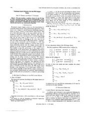
respectively. Table lists the theoretical voltage stress and
output line-to-line rms voltage based on the previous analysis.
Table . Theoretical voltage stress and output voltage under different
conditions
Operating
condition
M = 0.812,
Vdc = 145V
M = 1,
Vdc= 250 V
M = 1.1,
Vdc = 250 V
Voltage stress
(V)
Output voltage VL-L
(V)
357 177
342 209
276 186
The simulation results in Figs. 9–11 are consistent with
the theoretical analysis, which verifies the previous analysis
and the control concept.
IAS 2004 145
0-7803-8486-5/04/$20.00 © 2004 IEEE

(V)
(V)
(V)
(A)
150.0
145.0
140.0
400.0
200.0
0.0
80.0
40.0
0.0
400.0
200.0
0.0
-200.0
-400.0
(V)
(V)
(V)
(A)
0.25 0.26 0.27 0.28 0.29
t(s)
260.0
255.0
250.0
245.0
240.0
400.0
200.0
0.0
40.0
0.0
400.0
200.0
0.0
-200.0
-400.0
Fig. 9 Simulation results with M = 0.8
0.15 0.16 0.17 0.18 0.19
t(s)
Fig. 10 Simulation results with M = 1
(V) : t(s)
Input
Voltage
V dc
(V) : t(s)
DC Link
Voltage
V pn
(A) : t(s)
Inductor
Current
IL (V) : t(s)
Load
Voltage
VLab (V) : t(s)
Input
Voltage
V dc
(V) : t(s)
DC Link
Voltage
V pn
(A) : t(s)
Inductor
Current
I L
(V) : t(s)
Load
Voltage
V Lab
The experimental results with the same operating
conditions are shown in Figs. 12, 13, and 14, respectively.
Based on these results, the experimental results agree with
the analysis and simulation results very well. The validity of the
control method is verified.
(V)
(V)
(V)
(A)
260.0
255.0
250.0
245.0
240.0
400.0
200.0
0.0
40.0
0.0
400.0
200.0
0.0
-200.0
-400.0
0.15 0.16 0.17 0.18 0.19
t(s)
Fig. 11 Simulation results with M = 1.1
V dc (200 V/div)
V PN (200 V/div)
I L1 (20 A/div)
v Lab (200 V/div)
(V) : t(s)
Input
voltage
V dc
(V) : t(s)
DC Link
Voltage
V pn
(A) : t(s)
Inductor
Current
I L
(V) : t(s)
Load
Voltage
V Lab
Fig. 12 Experimental results with Vdc = 145V and M=0.812
V dc (200 V/div)
V PN (200 V/div)
I L1 (20 A/div)
v Lab (200 V/div)
Fig. 13 Experimental results with Vdc = 250V and M = 1
IAS 2004 146
0-7803-8486-5/04/$20.00 © 2004 IEEE

V dc ( 300 V/div )
V PN ( 200 V/div )
I L1 ( 20A /div )
v Lab ( 200 V/div )
Fig. 14 Experimental results with Vdc = 250V and M = 1.1
CONCLUSION
Two control methods to obtain maximum voltage gain
with constant boost have been presented that achieve
maximum voltage boost without introducing any
low-frequency ripple related to the output frequency. The
relationship of the voltage gain and the modulation index was
analyzed in detail. The different control methods have been
compared. The proposed method can achieve the minimum
passive components requirement and maintain low voltage
stress at the same time. The control method has been verified
by simulation and experiments.
REFERENCES
[1] F. Z. Peng, “Z-Source Inverter,” IEEE Transactions on Industry
Applications, 39(2), pp. 504–510, March/April 2003.
[2] F. Z. Peng and Miaosen Shen, Zhaoming Qian, “Maximum Boost Control
of the Z-source Inverter,” in Proc. of IEEE PESC 2004.
[3] D.A. Grant and J. A. Houldsworth: PWM AC Motor Drive Employing
Ultrasonic Carrier. IEE Conf. PE-VSD, London, 1984, pp. 234-240.
[4] Bimal K. Bose, Power Electronics and Variable Frequency Drives, Upper
Saddle River, NJ: Prentice-Hall PTR, 2002.
[5] P. T. Krein, Elements of Power Electronics, London, UK: Oxford Univ.
Press, 1998.
[6] W. Leonard, Control of Electric Drives, New York: Springer-Verlag,
1985
IAS 2004 147
0-7803-8486-5/04/$20.00 © 2004 IEEE