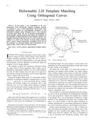
Acrobat (.pdf)

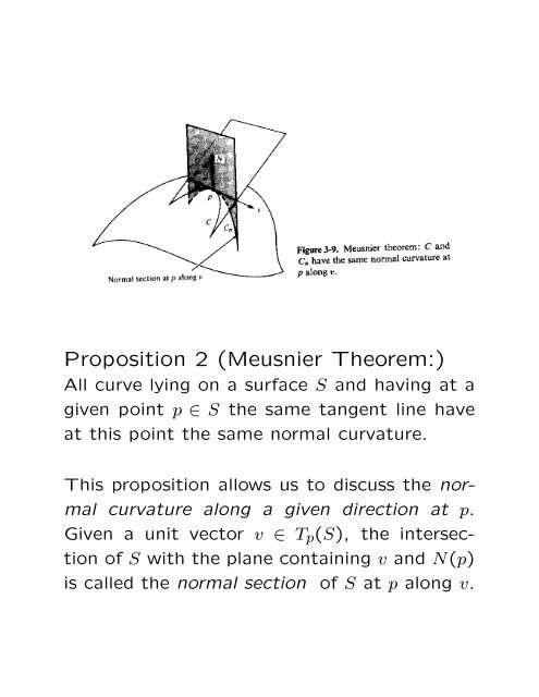
Proposition 2 (Meusnier Theorem:)
All curve lying on a surface S and having at a
given point p ∈ S the same tangent line have
at this point the same normal curvature.
This proposition allows us to discuss the normal
curvature along a given direction at p.
Given a unit vector v ∈ Tp(S), the intersection
of S with the plane containing v and N(p)
is called the normal section of S at p along v.

Given a self-adjoint linear map A : V → V ,
there exists an orthonormal basis for V such
that relative to that basis the matrix of A is
a diagonal matrix. Furthermore, the elements
on the diagonal are the maximum and the minimum
of the corresponding quadratic form restricted
to the unit circle of V .

For each p ∈ S, there exists an orthonormal basis
{e1, e2} of Tp(S) such that dNp(e1) = −k1e1,
dNp(e2) = −k2e2. Moreover, k1 and k2 (k1 ≥
k2) are the maximum and minimum of the second
fundamental for IIp restricted to the unit
circle of Tp(S); that is, they are the extreme
values of the normal curvature at p.
Definition 7:
The maximum normal curvature k1 and the
minimum normal curvature k2 are called the
principal curvatures at p; the corresponding directions,
that is, the directions given by the
eigenvectors e1 and e2, are called the principal
directions at p.

The knowledge of the principal curvatures at
p allows us to compute the normal curvature
along a given direction of Tp(S). Let v ∈ Tp(S)
with |v| = 1, and since e1 and e2 form an orthonormal
basis of Tp(S), we have
v = e1cosθ + e2sinθ
where θ is the angle from e1 to v in the orientation
of Tp(S). The normal curvature kn
along v is given by the Euler formula:
kn = IIp(v) = − < dNp(v), v >
= − < dNp(e1cosθ + e2sinθ), e1cosθ + e2sinθ >
= < e1k1cosθ + e2k2sinθ, e1cosθ + e2sinθ >
= k1cos 2 θ + k2sin 2 θ
The Euler formula is just the expression of the
second fundamental form in the basis {e1, e2}.

Definition 8:
Let p ∈ S and let dNp : Tp(S) → Tp(S) be the
differential of the Gauss map. The determinant
of dNp is the Gaussian curvature K of S
at p. The negative of half of the trace of dNp
is called the mean curvature H of S at p.
In term of the principal curvatures, we have
K = k1k2
H = k1 + k2
2

Definition 9:
A point of a surface S is called:
• Elliptic: if det(dNp) > 0.
• Hyperbolic: if det(dNp) < 0.
• Parabolic: if det(dNp) = 0, with dNp = 0.
• Planar: if dNp = 0.
Definition 10:
If at p ∈ S, k1 = k2, then p is called an umbilical
point of S; in particular, the planar points are
umbilical points.

Definition 11 (Dupin indicatrix):
Let p be a point in S. The Dupin indicatrix
at p is the set of vectors w of Tp(S) such that
IIp(w) = ±1.
In more convenient form, let (ξ, η) be the Cartesian
coordinates of Tp(S) in the orthonormal
basis {e1, e2}, where e1 and e2 are eigenvectors
of dNp. Given w ∈ Tp(S), let ρ and θ be
the polar coordinates defined by w = ρv, with
|v| = 1 and v = e1cosθ + e2sinθ if ρ = 0. By
Euler formula,
±1 = IIp(w) = ρ 2 IIp(v)
= k1ρ 2 cos 2 θ + k2ρ 2 sin 2 θ
= k1ξ 2 + k2η 2
where w = ξe1 + ηe2. Hence, the Dupin indicatrix
is a union of conics in Tp(S).

• For an elliptic point, the Dupin indicatrix is
an ellipse, and it degenerates into a circle
if the point is an umbilical nonplanar point
(k1 = k2 = 0).
• For a hyperbolic point, the Dupin indicatrix
is made up of two hyperbolas with a common
pair of asymptotic lines (zero normal
curvature).
• For a parabolic point, the Dupin indicatrix
degenerates into a pair of parallel lines.

Definition 12:
Let p be a point in S. An asymptotic direction
of S at p is a direction of Tp(S) for which the
normal curvature is zero. An asymptotic curve
of S is a regular connected curve C ⊂ S such
that for each p ∈ C the tangent line of C at p
is an asymptotic direction.
Definition 13:
Let p be a point in S. Two nonzero vectors
w1, w2 ∈ Tp(S) are conjugate if < dNp(w1), w2 >=<
w1, dNp(w2) >= 0. Two directions r1, r2 at
p are conjugate if a pair of nonzero vectors
w1, w2 parallel to r1 and r2, respectively, are
conjugate.

Gauss Map in Local Coordinates
From here on, all parameterizations x : U ⊂
R 2 → S are assumed to be compatible with
the orientation N of S; that is, in x(U),
N = xu × xv
|xu × xv|
Let x(u, v) be a parameterization at a point
p ∈ S, and let α(t) = x(u(t), v(t)) be a parameterized
curve in S, with α(0) = p.

The tangent vector to α(t) at p is
and
α ′ = xuu ′ + xvv ′
dN(α ′ ) = N ′ (u(t), v(t)) = Nuu ′ + Nvv ′
Since Nu and Nv belong to Tp(S), we may write
and therefore
Nu = a11xu + a21xv
Nv = a12xu + a22xv
dN(α ′ ) = (a11u ′ + a12v ′ )xu + (a21u ′ + a22v ′ )xv
hence,
dN
u ′
v ′
=
a11 a12
a21 a22
This shows that in the basis {xu, xv}, dN is
given by the matrix (aij) which is not necessarily
symmetric, unless {xu, xv} is an orthonormal
basis.
u ′
v ′

In the basis {xu, xv}, the second fundamental
form is given by
IIp(α ′ ) = − < dN(α ′ ), α ′ >
= − < Nuu ′ + Nvv ′ , xuu ′ + xvv ′ >
= e(u ′ ) 2 + 2fu ′ v ′ + g(v ′ ) 2
where, since < N, xu >=< N, xv >= 0,
e = − < Nu, xu >=< N, xuu >
f = − < Nv, xu >=< N, xuv >= − < Nu, xv >
g = − < Nv, xv >=< N, xvv >

Weingarten Mapping:
The matrix [β] = (aij) in the form
[β] = −
e f
f g
E F
F G
−1
is called the Weingarten mapping matrix or the
shape operator matrix of the surface. This matrix
combines the first and second fundamental
forms into one matrix, and determines surface
shape by relating the intrinsic geometry of the
surface to the Euclidean (extrinsic) geometry
of the embedding space.
The Gaussian curvature of a surface can be
obtained from the Weingarten mapping matrix
as its determinant:
eg − f 2
K = det[β] =
EG − F 2
And the mean curvature is similarly half of the
trace of the Weingarten mapping matrix:
H = tr[β]
2
= eG − 2fF + gE
2(EG − F 2 )

Koenderink Shape Index:
The signs of the Gaussian, mean and principal
curvatures are often used to determine basic
surface types and singular points such as
umbilical points. Furthermore, the numerical
relationship between the two principal curvatures
are used in more detailed classification
of surfaces by Koenderink, where a shape index
function is defined as
si = 2
π arctanκ2 + κ1
, (κ2 ≥ κ1)
κ2 − κ1
This way, all surface patches, except for plane
patches where the two principal curvatures equal
zero, are mapped onto si ∈ [−1, +1]. This
shape index function has many nice properties
with regards to the classification of surface
types:
• The shape index is scale invariant, i.e. two
spherical patches with different radii will
have same shape index values.

• Convexities and concavities are on the opposite
sides of the shape index scale, separated
by saddle-like shapes.
• Two shapes from which the shape index
differs only in sign represent complementary
pairs will fit to each other as stamp
and mold if they are of same scale.

spherical trough rut saddle saddle saddle ridge dome spherical
cup rut ridge cap
Surface Type Shape Index Range
Spherical Cup si ∈ [−1, −7/8)
Trough si ∈ [−7/8, −5/8)
Rut si ∈ [−5/8, −3/8)
Saddle Rut si ∈ [−3/8, −1/8)
Saddle si ∈ [−1/8, +1/8)
Saddle Ridge si ∈ [+1/8, +3/8)
Ridge si ∈ [+3/8, +5/8)
Dome si ∈ [+5/8, +7/8)
Spherical Cap si ∈ [+7/8, +1]

Shape Characterization of Discrete
Surfaces
For a regular surface S ⊂ R 3 and p ∈ S, there
always exists a neighborhood V of p in S such
that V is the graph of a differentiable function
which has one of the following three forms:
z = h(x, y)
y = s(x, z)
x = t(y, z)
Hence, given a point p of a surface S, we can
choose the coordinate axis of R 3 such that the
origin O of the coordinates is at p and the z
axis is directed along the outward normal of
S at p (thus, the xy plane agrees with the
tangent plane Tp(S)). It follows that a neighborhood
of p in S can be represented in the
form z = h(x, y), (x, y) ∈ U ⊂ R 2 , where U is
an open set and h is a differentiable function,
with h(0, 0) = 0, hx(0, 0) = 0, hy(0, 0) = 0.

In this case, the local surface is parameterized
by
x(u, v) = (u, v, h(u, v)), (u, v) ∈ U
where u = x, v = y. It can be shown that
xu = (1, 0, hu)
xv = (0, 1, hv)
xuu = (0, 0, huu)
xuv = (0, 0, huv)
xvv = (0, 0, hvv)
Thus, the normal vector at (x, y) is
N(x, y) = (−hx, −hy, 1)
(1 + h 2 x + h2 y )1/2

From the above expressions, it is easy to obtain
the coefficients of the first and second
fundamental forms as
E(x, y) = 1 + h 2 x
F (x, y) = hxhy
G(x, y) = 1 + h 2 y
e(x, y) =
f(x, y) =
g(x, y) =
hxx
(1 + h 2 x + h2 y )1/2
hxy
(1 + h 2 x + h 2 y) 1/2
hyy
(1 + h 2 x + h2 y )1/2
Hence, the curvatures of the surface can be
derived from the Weingarten mapping matrix
computed from these coefficients.