Pulsed-field gradient nuclear magnetic resonance as a tool for ...
Pulsed-field gradient nuclear magnetic resonance as a tool for ...
Pulsed-field gradient nuclear magnetic resonance as a tool for ...

Create successful ePaper yourself
Turn your PDF publications into a flip-book with our unique Google optimized e-Paper software.
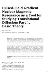
<strong>Pulsed</strong>-Field Gradient<br />
Nuclear Magnetic<br />
Resonance <strong>as</strong> a Tool <strong>for</strong><br />
Studying Translational<br />
Diffusion: Part II.<br />
Experimental Aspects<br />
WILLIAM S. PRICE<br />
Water Research Institute, Sengen 2-1-6, Tsukuba, Ibaraki 305-0047, Japan; E-mail: wprice@wri.co.jp<br />
ABSTRACT: In Part 1 of this series, we considered the theoretical b<strong>as</strong>is behind the<br />
pulsed-<strong>field</strong> <strong>gradient</strong> <strong>nuclear</strong> <strong>magnetic</strong> <strong>resonance</strong> method <strong>for</strong> me<strong>as</strong>uring diffusion. In this<br />
article the experimental and practical <strong>as</strong>pects of conducting such experiments are considered,<br />
including technical problems involved in <strong>gradient</strong> production such <strong>as</strong> eddy currents,<br />
<strong>gradient</strong> calibration, internal <strong>gradient</strong>s in heterogeneous samples, and temperature control.<br />
Furthermore, the means <strong>for</strong> recognizing and preventing or at le<strong>as</strong>t minimizing these<br />
problems are discussed. A number of representative pulse sequences are also reviewed.<br />
1998 John Wiley & Sons, Inc. Concepts Magn Reson 10: 197 237, 1998<br />
KEY WORDS: background <strong>gradient</strong>; diffusion; eddy currents; <strong>gradient</strong> calibration; pulsed<br />
<strong>field</strong> <strong>gradient</strong><br />
INTRODUCTION: PERFORMING A<br />
SIMPLE PULSED-FIELD GRADIENT ( PFG)<br />
NUCLEAR MAGNETIC RESONANCE<br />
( NMR) MEASUREMENT<br />
In the first article Ž 1. of this series Žreferred<br />
to<br />
here <strong>as</strong> Part 1. on PFG NMR <strong>as</strong>o<br />
known <strong>as</strong><br />
pulsed-<strong>gradient</strong> spin-echo Ž PGSE. NMR diffu-<br />
Received 12 December 1997; revised 5 February<br />
1998; accepted 6 February 1998.<br />
Concepts in Magnetic Resonance, Vol. 10Ž. 4 197237 Ž 1998.<br />
1998 John Wiley & Sons, Inc. CCC 1043-734798040197-41<br />
sion me<strong>as</strong>urements, we considered in detail the<br />
underlying principles of the PFG NMR experiment<br />
Ž Figure 1. and presented the b<strong>as</strong>ic mathematical<br />
analysis required to analyze the results of<br />
such experiments. This article expands the first<br />
one by considering the experimental <strong>as</strong>pects and<br />
complications.<br />
Let us begin by <strong>as</strong>suming that we have a simple<br />
liquid sample such <strong>as</strong> H 2Oor CCl 4 where<br />
there is only one species, and that we wish to<br />
me<strong>as</strong>ure its diffusion coefficient, D, using the<br />
simple Hahn spin-echob<strong>as</strong>ed PFG pulse sequence<br />
Ž i.e., the Stejskal and Tanner sequence.<br />
197
198<br />
PRICE<br />
Figure 1 The Stejskal and Tanner pulsed-<strong>field</strong> <strong>gradient</strong><br />
NMR sequence. The principles of this sequence <strong>for</strong><br />
me<strong>as</strong>uring diffusion were presented in Part 1. This is<br />
the simplest pulse sequence <strong>for</strong> me<strong>as</strong>uring diffusion.<br />
Ph<strong>as</strong>e cycling can be included to remove spectrometer<br />
artifacts. We have indicated the second half of the<br />
echo by dots, <strong>as</strong> it is this part of the echo Ži.e.,<br />
starting<br />
at t 2. that is digitized and used <strong>as</strong> the FID.<br />
shown in Fig. 1. To per<strong>for</strong>m this sequence, the<br />
spectrometer must be equipped with a current<br />
amplifier, under software control, which can send<br />
current pulses to a <strong>gradient</strong> coil placed around<br />
the sample Ž Fig. 2 . . Since this simple sequence is<br />
b<strong>as</strong>ed on a Hahn spin-echo, the echo signal, S, is<br />
attenuated by both the effects of the spinspin<br />
relaxation and of diffusion. As shown in Part 1<br />
Ž .<br />
1 , the signal intensity is given by<br />
2<br />
SŽ 2. SŽ 0. expž T / 2<br />
<br />
attenuation due<br />
to relaxation<br />
Ž 2 2 2 Ž ..<br />
exp g D 3<br />
<br />
attenuation due<br />
to diffusion<br />
Ž . Ž 2 2 2 Ž ..<br />
S 2 exp g D 3<br />
g0<br />
<br />
1<br />
where SŽ. 0 is the signal immediately after the<br />
2 pulse, 2 is the total echo time, T2 is the<br />
spinspin relaxation time of the species, is<br />
the gyro<strong>magnetic</strong> ratio of the observe nucleus, g<br />
is the strength of the applied <strong>gradient</strong>, and and<br />
are the duration of the <strong>gradient</strong> pulses and the<br />
separation between them, respectively. Typically,<br />
is in the range of 010 ms, is in the range of<br />
milliseconds to seconds and g is up to 20 T m1 .<br />
To remove the effects of the signal attenuation<br />
due to, in the c<strong>as</strong>e of the Stejskal and Tanner<br />
sequence, spinspin relaxation, we normalize the<br />
signal with respect to the signal obtained in the<br />
absence of the applied <strong>gradient</strong> and thereby define<br />
the echo attenuation to be<br />
Ž .<br />
E 2 <br />
Ž . Ž 2 2 2 Ž ..<br />
S 2 exp g D 3<br />
g0<br />
Ž .<br />
S 2 g0<br />
Ž 2 2 2 Ž .. <br />
exp g D 3 2<br />
By inspection of Eq. 2 with reference to Fig. 1, it<br />
can be seen that to me<strong>as</strong>ure diffusion, a series of<br />
experiments are per<strong>for</strong>med in which either g, ,<br />
or is varied while keeping constant. Then,<br />
Eq. 2 is regressed onto the experimental data<br />
and D is straight<strong>for</strong>wardly determined <strong>as</strong> discussed<br />
in Part 1.<br />
Un<strong>for</strong>tunately, the above description pertains<br />
only to per<strong>for</strong>ming the diffusion me<strong>as</strong>urements<br />
under ideal conditions, and includes the following<br />
implicit <strong>as</strong>sumptions: Ž. a the <strong>gradient</strong> pulses are<br />
perfectly rectangular Ži.e.,<br />
infinitely f<strong>as</strong>t rise and<br />
fall times . , Ž b. the <strong>gradient</strong> pulses are equally<br />
matched and of known strength, Ž. c the only<br />
<strong>magnetic</strong> <strong>field</strong> <strong>gradient</strong>s present are the applied<br />
<strong>gradient</strong> pulses, Ž d. all of the sample is subject to<br />
exactly the same <strong>gradient</strong>, Ž. e all of the sample is<br />
at exactly the same temperature, and Ž. f the relaxation<br />
characteristics of the sample do not constrain<br />
the choice of or the recycle time of the<br />
pulse sequence. In a real experiment, all of these<br />
points must be addressed, or at le<strong>as</strong>t their significance<br />
understood. These points are considered in<br />
this article.<br />
Although few researchers will attempt to construct<br />
their own equipment since the requisite<br />
<strong>gradient</strong> hardware is now commercially available,<br />
a b<strong>as</strong>ic understanding of <strong>gradient</strong> pulse generation<br />
provides valuable insight into spectrometer<br />
limitations and related problems. Accordingly, in<br />
the next section we will briefly consider the hardware<br />
required to generate <strong>magnetic</strong>-<strong>field</strong> <strong>gradient</strong><br />
pulses and what levels of per<strong>for</strong>mance are required<br />
<strong>for</strong> conducting diffusion experiments.<br />
Hardware problems and the experimental ramifications<br />
of imperfect <strong>gradient</strong> pulses will be considered<br />
in the third section. Sample preparation<br />
and spectrometer setup will be considered in the<br />
fourth section. Problems relating directly to<br />
the sample and their solutions are discussed in<br />
the fifth section. In the penultimate section, the<br />
methods <strong>for</strong> calibrating the applied <strong>gradient</strong> are<br />
considered; and finally, in the l<strong>as</strong>t section, a summary<br />
of how to conduct PFG experiments is presented.<br />
As in our previous article, we will confine<br />
ourselves to the more commonly used PFG exper-
PULSED-FIELD GRADIENT NMR: EXPERIMENTAL ASPECTS 199<br />
Figure 2 A schematic diagram of the components necessary to per<strong>for</strong>m pulsed-<strong>field</strong><br />
<strong>gradient</strong> NMR and their relationship to the rest of the spectrometer. At the appropriate<br />
points in the pulse sequence, the spectrometer sends logic pulses or Žon<br />
more sophisticated<br />
machines. shaped voltage pulses Ž wave<strong>for</strong>ms. such <strong>as</strong> trapezoidal pulses or pulses with<br />
pre-emph<strong>as</strong>is to the current amplifier. The current amplifier is, in turn, connected to the<br />
<strong>gradient</strong> coils placed around the sample in the probe head Ž Fig. 4 . . Sophisticated hardware<br />
will also allow the polarity of the <strong>gradient</strong> pulses to be specified, thus af<strong>for</strong>ding the<br />
possibility of per<strong>for</strong>ming pulse sequences with bipolar <strong>gradient</strong> pulses. More advanced<br />
spectrometers also include current blanking circuitry which prevents earth loops and thereby<br />
helps to minimize background <strong>gradient</strong>s. In this c<strong>as</strong>e, the current pulse circuitry is blanked<br />
out between <strong>gradient</strong> pulses.<br />
iments b<strong>as</strong>ed on <strong>magnetic</strong> <strong>field</strong> Ž i.e., B . 0 <strong>gradient</strong>s.<br />
It is appropriate to mention that many of<br />
the complications that affect PFG me<strong>as</strong>urements<br />
also apply to imaging experiments; consequently,<br />
some of the solutions to the technical problems<br />
were developed with imaging in mind Ž. 2 .<br />
HARDWARE<br />
Introduction<br />
The hardware <strong>as</strong>pects of PFG NMR have been<br />
discussed by a number of authors Že.g.,<br />
Refs.<br />
27 . , and <strong>for</strong> the present purposes it is sufficient<br />
to provide a b<strong>as</strong>ic overview. The additional hardware<br />
that must be added to a spectrometer to<br />
generate <strong>gradient</strong> pulses is summarized in Fig. 2.<br />
Specifically, the spectrometer, in accordance with<br />
the pulse sequence, needs to output either a logic<br />
pulse Ž if only rectangular pulses are required. or<br />
a shaped voltage pulse Žthereby<br />
af<strong>for</strong>ding the<br />
possibility of shaped <strong>gradient</strong> pulses. to an amplifier.<br />
Ideally, the polarity of the <strong>gradient</strong> pulse will<br />
also be able to be specified. In turn, the amplifier<br />
outputs a corresponding current pulse to the <strong>gradient</strong><br />
coil.<br />
Gradient Coils<br />
Many <strong>gradient</strong> coil designs exist Ž see Refs. 68 . ;<br />
however, we will restrict our discussion to the<br />
simplest commonly used geometry <strong>for</strong> producing<br />
<strong>gradient</strong>s along the z direction in superconducting<br />
magnets: the Maxwell pair of coils Ži.e.,<br />
anti-<br />
Helmholtz. Fig. 3Ž A ..<br />
The <strong>magnetic</strong> <strong>field</strong> strength<br />
at a point P Ž r , z . Ž Fig. 3. from a single<br />
p p
200<br />
PRICE<br />
FIGURE 3 Ž A. A schematic depiction of a cross-section through a Maxwell pair; this is a <strong>gradient</strong> coil <strong>for</strong> producing a <strong>gradient</strong> along<br />
the long axis of the coil and is the b<strong>as</strong>is of most <strong>gradient</strong> coils <strong>for</strong> producing z-axis <strong>gradient</strong>s in superconducting magnets. It should be<br />
noted that each set of windings h<strong>as</strong> an opposite handedness. In computing the <strong>gradient</strong> using Eqs. 3 and 4 , the coil radius rc is<br />
adjusted according to the actual winding being calculated. The <strong>gradient</strong> g z at a point P is calculated by computing the <strong>magnetic</strong> <strong>field</strong> at<br />
two points separated by a distance along the z axis, zd, Ži.e., P Ž r , z zd2. and P Ž r , z zd2 .<br />
1 p p 2 p p , denoted by the smaller solid<br />
circles. and dividing by the distance between them. Ž B. A contour plot of the <strong>gradient</strong> in the shaded region of the <strong>gradient</strong> coil depicted<br />
in Ž A. taking rc to be 0.6 cm, lc to be 3 cm, the wire diameter to be 0.5 mm, and I 1 A. The numbers on the contours denote the<br />
1 Ž 1 1<br />
<strong>gradient</strong> strength in G cm n.b., 1 G cm 0.01 T m . . Because this is a very simplistic design <strong>for</strong> a <strong>gradient</strong> coil, the volume having<br />
a constant Ž i.e., linear. <strong>gradient</strong> is very small. Ideally, the sample would be restricted to a volume with high <strong>gradient</strong> linearity Že.g.,<br />
the<br />
d<strong>as</strong>hed box . .
winding can be estimated from the BiotSavart<br />
Ž .<br />
law 9, 10 ,<br />
I 1<br />
0 p p<br />
0<br />
2 2<br />
Ž 2<br />
r . crp zp<br />
12<br />
Ž .<br />
B r , z <br />
where<br />
ž /<br />
½ 5<br />
r2r2z2 c p p<br />
KŽ u. EŽ u.<br />
2<br />
Ž . 2<br />
r r z<br />
c p p<br />
) 4rcrp Ž . 2<br />
r r z<br />
u 2<br />
c p p<br />
K and E are the elliptic integrals of the first and<br />
second kinds, respectively Ž 11 . . 0 is the permitivity<br />
constant, rp is the radius of the point at which<br />
the <strong>gradient</strong> is calculated, rc is the radius of the<br />
<strong>gradient</strong> coil, and zp is the displacement along<br />
the z axis from the coil Ž Fig. 3 . . The <strong>gradient</strong><br />
at P can then be computed by calculating the<br />
<strong>magnetic</strong> <strong>field</strong> strength at two points separated<br />
by a distance along the z axis, zd Ži.e.,<br />
P1 <br />
Ž r , z zd2 . , and P Ž r , z zd2 ..<br />
p p 2 p p , and<br />
dividing by the distance between the two points,<br />
coil<br />
windings<br />
g <br />
z, P<br />
ž / ž /<br />
zd zd<br />
B r , z B r , z <br />
2 2<br />
Ý 0 p p 0 p p<br />
zd<br />
PULSED-FIELD GRADIENT NMR: EXPERIMENTAL ASPECTS 201<br />
<br />
3<br />
In calculating Eq. 4 , it must be remembered that<br />
the sum runs over both windings of the Maxwell<br />
pair, and owing to the opposite polarity, one coil<br />
winding is taken <strong>as</strong> negative. Ideally, the <strong>gradient</strong><br />
coils should produce a perfectly constant Žor<br />
commonly<br />
termed ‘‘linear’’ . <strong>gradient</strong>, but owing to the<br />
space constraints inside the probe and inherent<br />
limitations in construction, such <strong>as</strong> attempting to<br />
produce a continuous <strong>magnetic</strong> <strong>field</strong> distribution<br />
from a finite number of turns Fig. 3Ž A .,<br />
the<br />
<strong>gradient</strong> coils never produce a perfectly constant<br />
<strong>gradient</strong>. A <strong>field</strong> plot <strong>for</strong> the <strong>gradient</strong> coils depicted<br />
in Fig. 3Ž A. is given in Fig. 3Ž B . .<br />
As will be explained in more detail below Žsee<br />
Eddy Currents and Perturbation of B . 0 , disturbances<br />
can result from the generation of eddy<br />
<br />
4<br />
currents in the conductors surrounding the <strong>gradient</strong><br />
coils owing to the rapid pulsing of the <strong>gradient</strong><br />
coils. The most direct solution to this problem<br />
is to limit the effects of the <strong>gradient</strong> pulse to the<br />
sample volume only. This is achieved by placing a<br />
shield <strong>gradient</strong> coil outside the Ž primary. <strong>gradient</strong><br />
coil Ž Fig. 4 . . Shielded <strong>gradient</strong> coils were originally<br />
proposed by Mans<strong>field</strong> and Chapman Ž12,<br />
13 . , Turner Ž 14 . , and Turner and Bowley Ž 15 . ,<br />
and the theoretical <strong>as</strong>pects of shielded <strong>gradient</strong><br />
coils have recently been summarized elsewhere<br />
Ž 2, 16 . . The shield coil is designed to prevent<br />
Ž i.e., cancel. the effects of the <strong>gradient</strong> pulse<br />
generated by the primary <strong>gradient</strong> coil radiating<br />
outward. Ideally, the change in the <strong>magnetic</strong> <strong>field</strong><br />
outside the <strong>gradient</strong> set due to the pulse would be<br />
zero, where<strong>as</strong> the <strong>gradient</strong> generated in the sample<br />
volume would be unaffected by the presence<br />
of the shield coil. In this way, no Žor<br />
at le<strong>as</strong>t<br />
greatly reduced. eddy currents are generated, typically<br />
to 1% Ž 17 . . We also note that these<br />
eddy current effects rapidly attenuate with incre<strong>as</strong>ing<br />
distance, and thus there is considerable<br />
advantage in using small <strong>field</strong> <strong>gradient</strong> coils in a<br />
wide-bore magnet. Importantly, after implementation,<br />
shielded <strong>gradient</strong> coils require no further<br />
experimental adjustment. A negative <strong>as</strong>pect of<br />
shielded <strong>gradient</strong> coils is that the shield coils<br />
decre<strong>as</strong>e the strength and linearity of the <strong>gradient</strong><br />
produced by the primary <strong>gradient</strong> coil Ž 18 . .It<br />
is possible to generate a profile of the <strong>gradient</strong><br />
strength by applying a read <strong>gradient</strong> during acquisition<br />
in the PFG sequence Ž 19. Žthis<br />
is related to<br />
the one-dimensional imaging method of calibrating<br />
the <strong>gradient</strong> strength discussed in Shape<br />
Analysis of the Spin Echo and One-Dimensional<br />
Images but retaining the <strong>gradient</strong> pulses <strong>for</strong> me<strong>as</strong>uring<br />
diffusion . . However, it h<strong>as</strong> been found in<br />
practice that a re<strong>as</strong>onable deviation from perfect<br />
linearity is allowable <strong>for</strong> many experiments Ž 20 . .<br />
A simple but tedious experimental means of testing<br />
the linearity of the <strong>gradient</strong> is to per<strong>for</strong>m<br />
diffusion me<strong>as</strong>urements using a very small sample<br />
at different positions within the volume where the<br />
sample would normally lie. A water sample in a<br />
small spherical bulb Ž e.g., Wilmad cat. no. 529A.<br />
is a convenient choice.<br />
Although most diffusion studies are per<strong>for</strong>med<br />
with a <strong>gradient</strong> in one dimension only, it is now<br />
incre<strong>as</strong>ingly common, especially with the advent<br />
of imaging and microscopy probes, to per<strong>for</strong>m<br />
diffusion experiments in three dimensions so <strong>as</strong>
202<br />
PRICE<br />
Figure 4 An example of a shielded <strong>magnetic</strong> <strong>gradient</strong> coil system in an NMR probe head.<br />
Only the coil <strong>for</strong>mers are shown, and the wires can be imagined to be wound around the<br />
slots on the <strong>for</strong>mers. The primary <strong>gradient</strong> coil produces the constant <strong>gradient</strong> over the<br />
sample volume which is contained within the rf coils. The shield coil is designed to prevent<br />
the <strong>gradient</strong> pulse from affecting outside the <strong>gradient</strong> coils, thereby preventing the generation<br />
of eddy currents adapted from Price et al. Ž 6 ..<br />
In very high <strong>gradient</strong> systems, the actual<br />
<strong>gradient</strong> coils must be air or water cooled. The position of the thermocouple is critical <strong>for</strong><br />
the accuracy and stability of the temperature control. The inclusion of <strong>gradient</strong> coils in the<br />
probe head normally makes the probe more difficult to shim.<br />
to obtain the diffusion tensor Žsee<br />
Part 1,<br />
Anisotropic Diffusion . .<br />
Amplifiers<br />
Ideally, we desire infinitely f<strong>as</strong>t rise and fall times<br />
of the <strong>gradient</strong> pulses. In practice, there are two<br />
factors which limit the maximum current switching<br />
speed; the first is that the power supply voltage<br />
must equal RI LdIdt, where I is the<br />
current and L and R are the load Ži.e.,<br />
<strong>gradient</strong><br />
coils plus leads. inductance and resistance, respectively,<br />
and the second is the slew rate Ži.e.,<br />
the maximum rate of change of the output voltage.<br />
of the power supply. Thus, the amplifier used<br />
must have suitable current and voltage parameters<br />
to drive the <strong>gradient</strong> coil used. Typically rise<br />
and fall times of the <strong>gradient</strong> pulses are on the<br />
order of 50 s.<br />
Since the current through a <strong>gradient</strong> coil induces<br />
heating, which in turn results in a change in<br />
<strong>gradient</strong> coil resistance, the amplitude of the gra-
dient pulses might change during the sequence.<br />
In fact, many <strong>gradient</strong> coils, especially when used<br />
with large currents or duty cycles, need to be air<br />
andor water cooled to prevent physical damage.<br />
Similarly, in conducting variable temperature diffusion<br />
me<strong>as</strong>urements, the g<strong>as</strong> used <strong>for</strong> heating<br />
and cooling the sample will also have some effect<br />
on the <strong>gradient</strong> coil temperature. The use of a<br />
constant current supply, instead of a constant<br />
voltage amplifier, obviates the need to calibrate<br />
the <strong>gradient</strong> <strong>for</strong> each sample temperature or particular<br />
experimental parameters. The negative <strong>as</strong>pects<br />
of a constant current amplifier are that it is<br />
difficult to achieve very low noise figures and<br />
rapid settling.<br />
HARDWARE PROBLEMS AND<br />
SOLUTIONS<br />
Sample Movement with Respect to the<br />
Gradient<br />
Mechanical stability is extremely important, since<br />
movements on the order of 10 nm will restrict<br />
15 2 1 Ž .<br />
diffusion me<strong>as</strong>urements to D 10 m s 21<br />
Že.g., see Part 1, Eq. 33 ,<br />
and consider the mean<br />
square displacement that occurs with such a diffusion<br />
coefficient and a typical value of such <strong>as</strong><br />
50 ms . . Sample movement is similar to flow in<br />
that all spins in the c<strong>as</strong>e of a rigid sample receive<br />
an equal ph<strong>as</strong>e shift Ž<strong>as</strong><br />
in the c<strong>as</strong>e of flow; see<br />
Part 1, Me<strong>as</strong>uring Diffusion with Magnetic Field<br />
Gradients. instead of a ph<strong>as</strong>e twist. Thus, <strong>as</strong>suming<br />
that the sample moves by r between the first<br />
and second <strong>gradient</strong> pulses of strength g and<br />
duration , then the net ph<strong>as</strong>e shift would be<br />
given by<br />
Ž .<br />
exp ig r<br />
movement<br />
Ž . <br />
exp i2q r 5<br />
Ž . 1<br />
where q 2 g.<br />
A string of equally spaced Ž i.e., by . <strong>gradient</strong><br />
pulses be<strong>for</strong>e the start of the pulse sequence may<br />
also help to alleviate motional disturbances during<br />
the encoding and decoding <strong>gradient</strong> pulses<br />
Ž 22. Ž see Fig. 8 . . Sample movement or vibration<br />
can result in greatly incre<strong>as</strong>ed echo attenuation<br />
Ž 23. and attenuation plots containing artifactual<br />
diffraction minima; however, these artifactual<br />
diffractive minima are evident at even modest<br />
attenuations, where<strong>as</strong> real diffractive minima Žsee<br />
Part 1, especially Fig. 8. generally do not become<br />
evident until the echo signal h<strong>as</strong> been attenuated<br />
PULSED-FIELD GRADIENT NMR: EXPERIMENTAL ASPECTS 203<br />
by nearly two orders of magnitude. To check <strong>for</strong><br />
the possibility of vibration, it is advisable to per<strong>for</strong>m<br />
a me<strong>as</strong>urement under the same conditions<br />
to be used experimentally with a very large monodisperse<br />
polymer Že.g.,<br />
polydimethylsiloxane, MW<br />
700 000 h<strong>as</strong> a diffusion coefficient below 10 15<br />
2 1 Ž ..<br />
ms 24 <strong>for</strong> which true diffractive peaks can-<br />
not occur and <strong>for</strong> which the diffusion coefficient<br />
is generally below the limits of me<strong>as</strong>urability Ž 25 . .<br />
If, <strong>as</strong>suming that the sample is correctly positioned<br />
in the probe, no attenuation is observed,<br />
the presence of artifacts can be excluded. However,<br />
this test does not account <strong>for</strong> independent<br />
movement of the sample with respect to the sample<br />
tube <strong>as</strong> might occur with a powder sample<br />
Ž e.g., zeolite. Ž 23 . . In such c<strong>as</strong>es, the samples may<br />
need to be specially compacted into the NMR<br />
tube Ž 23 . . If the me<strong>as</strong>ured diffusion coefficient is<br />
observed to be observation time independent Žal<br />
though must be sufficiently small so that the<br />
effects of restricted diffusion are insignificant . ,<br />
artifacts due to sample instability can be excluded.<br />
( )<br />
Radiofrequency rf Coupling<br />
The addition of <strong>gradient</strong> coils to an NMR probe<br />
generally h<strong>as</strong> a deleterious effect on general probe<br />
per<strong>for</strong>mance. Although with modern commercially<br />
obtainable equipment this is becoming less<br />
of an issue, we mention the effects here <strong>for</strong><br />
completeness. Partly owing to the proximity of<br />
the <strong>gradient</strong> coils to the sample region, the <strong>gradient</strong><br />
coils and leads have the possibility of acting<br />
<strong>as</strong> antennae and introducing rf interference. In<br />
fact, the present author h<strong>as</strong> also observed the<br />
heater cable to be a source of rf interference. The<br />
presence of rf interference can be tested <strong>for</strong> by<br />
observing a spectrum<strong>for</strong> example, after a 2<br />
pulseand then disconnecting the <strong>gradient</strong> current<br />
leads and acquiring another spectrum. The rf<br />
interference will appear <strong>as</strong> spikes andor general<br />
noise. It h<strong>as</strong> been the present author’s experience<br />
that frequencies below 200 MHz are more problematic<br />
<strong>for</strong> this kind of interference. Apart from<br />
simply collecting a far greater number of scans to<br />
obtain sufficient signal-to-noise, the best solution<br />
is to employ rf filtering on these sources of interference.<br />
A related problem is the possible strong<br />
mutual inductance between the <strong>gradient</strong> and the<br />
rf coils. Thus, the Q of the rf coilŽ. s are diminished,<br />
resulting in longer 2 pulses, poorer decoupling<br />
efficiency, and a poorer signal-to-noise<br />
ratio.
204<br />
PRICE<br />
Amplifier Noise, Earth Loops, and<br />
Nonreproducible ( Mismatched)<br />
Gradient Pulses<br />
In this section, we consider the effects introduced<br />
by unintended currents flowing through the <strong>gradient</strong><br />
system resulting in background <strong>gradient</strong>s.<br />
The problems resulting directly from the <strong>gradient</strong><br />
pulses themselves are discussed in the next<br />
section.<br />
In the absence of <strong>gradient</strong> pulses, there should<br />
be zero current flowing through the <strong>gradient</strong> coils;<br />
however, in practice slight differences in potential<br />
difference between different parts of the spectrometer<br />
Že.g.,<br />
the amplifier and the input line<br />
may not have the same zero voltage. cause currents<br />
to flow through the <strong>gradient</strong> coils between<br />
pulses, resulting in nonrandom <strong>gradient</strong>s. Similarly,<br />
the amplifier will also have a noise level<br />
resulting in small currents through the coils. Although<br />
very small, such earth loop and noise<br />
currents result in troublesome background <strong>gradient</strong>s<br />
and can completely thwart high-resolution<br />
diffusion experiments, since they will be present<br />
during signal acquisition Žsimilar<br />
to bad shimming.<br />
<strong>as</strong> well <strong>as</strong> attenuating the signal <strong>as</strong> in the<br />
normal Hahn spin-echo sequence Žsee<br />
Part 1, Eq.<br />
17 . . Ideally, one would have an oscilloscope<br />
available when tracing noise problems on a spectrometer,<br />
but the observed spectrum itself <strong>for</strong>ms<br />
an extremely sensitive probe. Earth loop currents<br />
can be detected by physically disconnecting the<br />
<strong>gradient</strong> circuit and looking at the effect on the<br />
line shape or shift of the signal in the observed<br />
spectrum, or, if available, by the effects on the<br />
lock signal. The effects of amplifier noise can be<br />
further <strong>as</strong>sessed by observing a spectrum with and<br />
without the amplifier turned on Žn.b.,<br />
with the<br />
inputs of the amplifier shorted . .<br />
To prevent the effects of earth loops and noise,<br />
all of the components in the spectrometer and<br />
current amplifier should be earthed to the same<br />
point, and ideally, the <strong>gradient</strong> coil should be<br />
blanked Ž i.e., disconnected. from the current circuit<br />
between <strong>gradient</strong> pulses Ž Fig. 2 . . Blanking,<br />
however, will not prevent the effects of noise<br />
during the <strong>gradient</strong> pulses. Very small earth loop<br />
effects can be shimmed out if the earth loop<br />
currents result in a steady <strong>gradient</strong>.<br />
Although the pulse program clearly defines<br />
when the spectrometer should send logic or<br />
shaped voltage pulses to the current amplifier, the<br />
logic line or shaped voltage line from the spectrometer<br />
to the amplifier may not be delivering<br />
clean pulses to the amplifier, and some degree of<br />
noise is common. This noise will, of course, be<br />
amplified by the amplifier resulting in <strong>gradient</strong><br />
noise Ž i.e., randomly changing <strong>gradient</strong>s . . This<br />
noise problem is compounded by the amplifier’s<br />
inherent noise level. The input noise can be detected<br />
by observing a spectrum be<strong>for</strong>e and after<br />
shorting the input to the <strong>gradient</strong> amplifier Žn.b.,<br />
the <strong>gradient</strong>s are not pulsed. and looking at the<br />
effect on the line shape or shift of the signal in<br />
the observed spectrum, or, if available, by the<br />
effects on the lock signal.<br />
Stable and perfectly reproducible <strong>gradient</strong><br />
pulses are crucial <strong>for</strong> accurate PFG me<strong>as</strong>urements.<br />
In a modern spectrometer, accurate timing<br />
of pulses and their duration is generally not a<br />
problem. The major sources of imprecision are, <strong>as</strong><br />
noted above, the noise in the <strong>gradient</strong> system, and<br />
it may not necessarily be uni<strong>for</strong>m with time and<br />
the instability of the amplifier. However, it h<strong>as</strong><br />
also been noted that the refocusing rf pulse Ži.e.,<br />
the pulse in the Stejskal and Tanner sequence.<br />
induces a signal in the <strong>gradient</strong> coils, which in<br />
turn elicits a small current pulse from the current<br />
amplifier Ž 26. Žalthough<br />
this problem can be<br />
overcome by a more sophisticated <strong>gradient</strong> driver<br />
design . . As we will discuss in detail below, the<br />
defocusing and refocusing effects of the <strong>gradient</strong><br />
pulses in the pulse sequence must be very finely<br />
matched. We note that the <strong>gradient</strong> magnitude<br />
needed to me<strong>as</strong>ure a dynamic displacement n<br />
orders of magnitude smaller than the sample dimensions<br />
will result in a deph<strong>as</strong>ing of order 10 n<br />
cycles across the sample and that the refocusing<br />
must be accurate to within a few degrees Žsee<br />
Fig. 2 of Part 1 . . Thus, <strong>for</strong> example, to me<strong>as</strong>ure a<br />
displacement of 0.1 m in a 5-mm tube, the<br />
<strong>gradient</strong> pulse pair must be matched to better<br />
5 than 1 in 10 Ž 2 . ; thus, the greater the stability<br />
and the lower the noise of the system, the better.<br />
We also note that the <strong>gradient</strong> pulses themselves<br />
contribute to the problem themselves owing to<br />
the generation of eddy currents; this will be discussed<br />
in detail in the next section. Thein some<br />
waysrelated effect of sample movement w<strong>as</strong><br />
considered in Sample Movement with Respect to<br />
the Gradient. As mentioned in Amplifiers, the<br />
effects of <strong>gradient</strong> coil heating are normally overcome<br />
by the use of a constant current amplifier.<br />
However, it may be that the amplifier is incapable<br />
of producing two equally matched <strong>gradient</strong> pulses<br />
in quick succession. A means of incre<strong>as</strong>ing the<br />
reproducibility of the pulses is to place additional,<br />
appropriately spaced Ž i.e., apart. <strong>gradient</strong> pulses
prior to the start of the rf pulse sequence see<br />
Fig. 8Ž B ..<br />
To illustrate the effects of imperfectly matched<br />
<strong>gradient</strong> pulses, we consider the Stejskal and Tanner<br />
pulse sequence. We recall from Part 1 that<br />
<strong>for</strong> a single nondiffusing spin at position z, and<br />
considering only the effects of the applied <strong>gradient</strong><br />
pulses Žwe denote g <strong>as</strong> gt Ž . to emph<strong>as</strong>ize the<br />
time dependence of the <strong>gradient</strong> pulse . , the cumulative<br />
ph<strong>as</strong>e shift at 2 is given by<br />
H H<br />
2 <br />
Ž 2. gŽ t. zdt gŽ t. zdt 6 0 <br />
and that the normalized intensity Ži.e.,<br />
an attenuation.<br />
of the echo signal at 2 is given by Ž 27, 28.<br />
Žsee Part 1, Eqs. 1012 . ,<br />
H<br />
<br />
SŽ 2. SŽ 2. PŽ ,2. cos d 7 g0 <br />
where SŽ 2. is the signal Ž<br />
g0<br />
i.e., resultant mag-<br />
netic moment. in the absence of a <strong>field</strong> <strong>gradient</strong><br />
and PŽ ,2. is the Ž relative. ph<strong>as</strong>e-distribution<br />
function which <strong>for</strong> the c<strong>as</strong>e of a single spin is<br />
equal to unity. From Eq. 7 , we can see that if<br />
0, the echo will be maximum and properly<br />
ph<strong>as</strong>ed. Thus, only if the <strong>gradient</strong> pulses are<br />
perfectly matched i.e.,<br />
the integral over the <strong>gradient</strong><br />
in the first period matches that in the<br />
second period ŽEq. . 6 will the echo maximum<br />
occur at t 2. If they do not, and acquisition is<br />
begun at t 2, the echo will not be in ph<strong>as</strong>e<br />
and its intensity will be reduced. If the degree of<br />
mismatch fluctuates, the position of the echo<br />
maximum will also fluctuate. In the c<strong>as</strong>e of an<br />
ensemble of spins at different positions, z, the<br />
magnetization helix Ž 29. will not be properly unwound<br />
Ži.e.,<br />
there will be a residual ph<strong>as</strong>e twist;<br />
consider the top series of spin ph<strong>as</strong>e diagrams in<br />
Fig. 2 of Part 1 . . Writing in terms of q, the ph<strong>as</strong>e<br />
twist resulting from a <strong>gradient</strong> pulse mismatch of<br />
q Žhere,<br />
denotes differential, not the delay in<br />
the pulse sequence. would be given by<br />
Ž . <br />
exp i2q r 8<br />
ph<strong>as</strong>e twist<br />
In the observed spectrum, the ph<strong>as</strong>e problem<br />
would not be evident and the observed signal<br />
intensity will be severely reduced, since the vector<br />
sum of the magnetization helix in the xy plane<br />
will be close to zero. Out of simplicity, we have<br />
PULSED-FIELD GRADIENT NMR: EXPERIMENTAL ASPECTS 205<br />
taken gt Ž. to reflect only the applied <strong>gradient</strong><br />
pulses; in reality, gt Ž. in Eq. 6 contains all<br />
<strong>gradient</strong>s present Ži.e.,<br />
noise <strong>gradient</strong>s, B0 imperfection,<br />
and internal <strong>gradient</strong>s . . The effects of<br />
internal <strong>gradient</strong>s will be considered in Short<br />
Relaxation Times, Internal Gradients, and Other<br />
Problems.<br />
The equation describing the echo attenuation<br />
<strong>for</strong> the Stejskal and Tanner sequence where the<br />
second <strong>gradient</strong> pulse is mismatched by a duration<br />
longer than the first pulse Ž Table 1. can be<br />
readily derived using the theory presented in the<br />
first article Žsee<br />
Part 1, The Macroscopic Approach.<br />
and is found to be Ž 30.<br />
Ž 2 2 2 Ž .<br />
Eexp g D 3<br />
2 Ž .4. <br />
2t 23 9<br />
1<br />
It can be seen that the mismatch introduces a <br />
and t1 dependence to the equation; interestingly,<br />
though, enters into the equation in second<br />
order Ž 31 . . However, where<strong>as</strong> the mismatch may<br />
have only a small effect on the attenuation due to<br />
the diffusion, the signal may be unobservably<br />
small.<br />
One solution to mismatched <strong>gradient</strong> pulses is<br />
to finely adjust the magnitude or Ž more e<strong>as</strong>ily. the<br />
duration of one of the <strong>gradient</strong> pulses with respect<br />
to the other Žsee,<br />
<strong>for</strong> example, Fig. 2 in Ref.<br />
32 . . For example, the Stejskal and Tanner sequence<br />
could first be per<strong>for</strong>med in the absence of<br />
<strong>gradient</strong> pulses and used to determine the reference<br />
ph<strong>as</strong>e setting. Subsequently, the same experiment<br />
could be per<strong>for</strong>med but using <strong>gradient</strong><br />
pulses. If the <strong>gradient</strong> pulses are perfectly<br />
matched, a maximum echo will occur at t 2.<br />
However, this is an empirical approach and is<br />
dependent on the experimental times and <strong>gradient</strong><br />
strengths used, and may not even be applica-<br />
( )<br />
Table 1 g t <strong>for</strong> the Stejskal and Tanner Sequence<br />
with Mismatched Gradient Pulses<br />
Ž.<br />
Subinterval of Pulse Sequence g t<br />
0 t t 0<br />
1<br />
t t t g<br />
1 1<br />
t tt 0<br />
1 1<br />
t tt g<br />
1 1<br />
t tt g<br />
1 1<br />
t t2 0<br />
1<br />
represents the degree of mismatch of the second <strong>gradient</strong><br />
pulse. If 0, then the sequence corresponds to that<br />
given in Fig. 1.
206<br />
PRICE<br />
ble if the source of the mismatch is due to eddy<br />
currentgenerated <strong>gradient</strong>s that are not parallel<br />
to the applied <strong>gradient</strong>s Ž 33. or nonconstant mismatch.<br />
We also note that the MASSEY sequence<br />
can be used to alleviate the ph<strong>as</strong>e-twist problem<br />
Ž see Postprocessing . . The ph<strong>as</strong>e-twist problem is<br />
considered in more detail in that section.<br />
Eddy Currents and Perturbation of B 0<br />
The rapid rise of the <strong>gradient</strong> pulses can generate<br />
eddy currents in the surrounding conducting surfaces<br />
around the <strong>gradient</strong> coils Že.g.,<br />
probe housing,<br />
cryostat, radiation shields, etc. . . The severity<br />
of the eddy current problem is thus proportional<br />
to dIdt and the strength of the <strong>gradient</strong>. Although<br />
the generation of eddy currents is greatly<br />
decre<strong>as</strong>ed through the use of shielded <strong>gradient</strong><br />
coils Ž see Gradient Coils . , they can still occur,<br />
especially when using large, rapidly rising and<br />
falling <strong>gradient</strong> pulses. The eddy currents, in turn,<br />
generate additional <strong>magnetic</strong> <strong>field</strong>s and thus have<br />
a close relationship to the problems discussed in<br />
the previous section. It is the decay of the eddy<br />
currents and their <strong>as</strong>sociated <strong>magnetic</strong> <strong>field</strong>s that<br />
determine the minimum delay that must be left<br />
between the end of the <strong>gradient</strong> pulse and the<br />
start of spectral acquisition. Eddy currents can<br />
have the following effects: Ž. a ph<strong>as</strong>e changes in<br />
the observed spectrum and anomalous changes in<br />
the attenuation, Ž b. <strong>gradient</strong>-induced broadening<br />
of the observed spectrum, and Ž. c time-dependent<br />
but spatially invariant B shift effects Ž<br />
0<br />
which appears<br />
<strong>as</strong> ringing in the spectrum . .<br />
We illustrate the effects of eddy currents using<br />
the Stejskal and Tanner sequence <strong>as</strong> an example.<br />
If the eddy current tail from the first <strong>gradient</strong><br />
pulse extends into the second -period, then the<br />
total <strong>field</strong> <strong>gradient</strong> during the second evolution<br />
period will not equal that in the first and the<br />
situation is analogous to the c<strong>as</strong>e of mismatched<br />
pulses see<br />
Amplifier Noise, Earth Loops, and<br />
Nonreproducible Ž Mismatched. Gradient Pulses .<br />
Consequently, even if a spin h<strong>as</strong> not moved in the<br />
direction of the <strong>gradient</strong> during the sequence,<br />
there will be a residual ph<strong>as</strong>e shift. As a result,<br />
the point at which the maximum echo appears<br />
will be shifted and its amplitude will be affected<br />
Ž 34 . . Thus, <strong>as</strong>suming that signal acquisition is<br />
begun <strong>as</strong> usual, at t 2 the eddy currents will<br />
cause additional attenuation unrelated to diffusion,<br />
and perhaps if the eddy currents have not<br />
dissipated be<strong>for</strong>e acquisition begins, ph<strong>as</strong>e shifts<br />
and spectral broadening.<br />
To gain some insight into the effects on the<br />
echo attenuation if the eddy currents generated<br />
by the first <strong>gradient</strong> pulse have not dissipated<br />
be<strong>for</strong>e the application of the pulse, and similarly,<br />
if the disturbances generated by the second<br />
<strong>gradient</strong> pulse have not dissipated prior to the<br />
start of acquisition, <strong>as</strong>suming infinitely f<strong>as</strong>t rise<br />
and but exponential fall Žwith<br />
exponential rate<br />
constant k. of the <strong>gradient</strong> pulses Ž Table 2 . , we<br />
can derive the echo attenuation equation <strong>for</strong> the<br />
Stejskal and Tanner sequence using the same<br />
method <strong>as</strong> be<strong>for</strong>e Žsee<br />
Part 1, The Macroscopic<br />
Approach . . An example program using the symbolic<br />
algebra package Maple Ž 35. is given in the<br />
Appendix Žn.b.,<br />
the new definition of the function<br />
F to allow <strong>for</strong> time-dependent <strong>gradient</strong>s . . The<br />
attenuation equation is given by<br />
Ž 2 2 2 Ž . Ž .4. <br />
Eexp g D 3 f t 10<br />
Table 2 g( t) <strong>for</strong> the Stejskal and Tanner Sequence in Which Eddy Currents Generated<br />
by the First Gradient Pulse Have Not Totally Decayed by the Time of Application of the<br />
Pulse ( A Similar Situation is Depicted in Fig. 5, if te Is Shorter Than the Time Required<br />
<strong>for</strong> the Eddy Current Effects to Dissipate) and Similarly the Eddy Currents from the<br />
Second Gradient Pulse Extending into the Acquisition Period<br />
Ž.<br />
Subinterval of Pulse Sequence g t<br />
0 t t 0<br />
1<br />
t t t g<br />
1 1<br />
t tt ge<br />
1 1<br />
t tt g<br />
1 1<br />
t t2 ge<br />
1<br />
k is the exponential rate constant.<br />
kŽtt .<br />
1<br />
kŽtt .<br />
1
where<br />
1<br />
Ž .<br />
2 2 kŽ.<br />
f t 2 e<br />
k ž<br />
<br />
kŽt1. 4e t1 <br />
2 /<br />
1<br />
2 kŽt1. Ž<br />
2 4e<br />
2 k<br />
kŽt 4 t e<br />
1.<br />
1<br />
2t 1<br />
Ž 2kŽ. kŽt e 4e 12. . .<br />
1<br />
Ž kŽt12. 8e 3 2k<br />
8ekŽ32t12. kŽ2t 4e 12.<br />
8e2kŽt1. 2kŽ.<br />
e<br />
2kŽ2t e 1. 1.<br />
This analysis is simplistic in the expression of the<br />
<strong>for</strong>m of the eddy currents and also because it<br />
does not consider the effects of the ph<strong>as</strong>e twist on<br />
the observed signal.<br />
Except <strong>for</strong> some c<strong>as</strong>es of restricted diffusion<br />
Ž . Ž . 2 2 2 36 , a plot of ln E versus g Ž 3. is<br />
normally linear in the c<strong>as</strong>e of free diffusion, or<br />
upward concave in the c<strong>as</strong>e of more complicated<br />
systems; von Meerwall and Kamat Ž 33. remarked<br />
that downward curvature is indicative of eddy<br />
current effects. Convection can also result in<br />
downward curvature.<br />
To determine if eddy current effects are significant,<br />
a me<strong>as</strong>urement can be per<strong>for</strong>med on a<br />
sample such <strong>as</strong> an extremely large monodisperse<br />
polymer with a diffusion coefficient lower than<br />
that which can be detected with the experimental<br />
system and parameters Ž i.e., , , and g. in question<br />
Ž see Gradient Calibration . . If the signal is<br />
attenuated or distorted, then the presence of eddy<br />
current effects is implied. Another simple way to<br />
determine if eddy current effects are present, and<br />
in particular to determine the minimum settling<br />
delay, t e,<br />
needed is to use the pulse sequence<br />
shown in Fig. 5 Ž 34 . . Some example spectra acquired<br />
using this pulse sequence are shown in<br />
Fig. 6. Eddy current <strong>field</strong>s can also be me<strong>as</strong>ured<br />
using search coils Ž 17 . , but such techniques are<br />
beyond the scope of the present article and are<br />
more commonly used in large imaging systems.<br />
Especially in the c<strong>as</strong>e of large <strong>gradient</strong>s, the<br />
rapid rise and fall of the pulses can directly affect<br />
the stability of the main <strong>magnetic</strong> <strong>field</strong> by induc-<br />
PULSED-FIELD GRADIENT NMR: EXPERIMENTAL ASPECTS 207<br />
Figure 5 A simple pulse sequence to determine the<br />
minimum time necessary <strong>for</strong> the effects of eddy currents<br />
to dissipate. In this sequence, a <strong>gradient</strong> pulse is<br />
first applied. After a delay t , an rf pulse Ž<br />
e<br />
not necessar-<br />
ily 2. is applied and a spectrum is acquired. Spectra<br />
are acquired with successively shorter te delays to<br />
determine the minimum time required <strong>for</strong> the eddy<br />
current effects to decay. Some examples of experimental<br />
spectra are shown in Fig. 6.<br />
ing additional currents into the solenoids producing<br />
the main <strong>magnetic</strong> <strong>field</strong>, or indirectly by affecting<br />
the lock feedback system. The final result<br />
is that the main <strong>field</strong> may be caused to oscillate<br />
or at le<strong>as</strong>t shift from its normal value Ži.e.,<br />
a<br />
time-dependent but spatially invariant B shift.<br />
0<br />
Ž 37 . . In such a c<strong>as</strong>e, if the ringing persists through<br />
acquisition, the observed spectrum will appear to<br />
be something like a spectrum observed with a<br />
continuous-wave NMR spectrometer.<br />
As noted above, shielded <strong>gradient</strong> coils may<br />
not sufficiently reduce the eddy currents generated<br />
in the surrounding conducting metals Žn.b.,<br />
they could still be generated in the rf coilif<br />
their design allows circulating low-frequency currents<br />
. . Eddy current problems are especially problematic<br />
when dealing with species with short T2 relaxation times, where it is impossible to sufficiently<br />
incre<strong>as</strong>e the delay after the <strong>gradient</strong> pulse<br />
to allow the eddy current effects to subside. Thus,<br />
we now consider further approaches <strong>for</strong> minimizing<br />
or coping with the effects of eddy currents.<br />
We can roughly divide the approaches into two<br />
categories: Ž. a hardware solutions, and Ž. b pulse<br />
sequence and postprocessing.<br />
Hardware Solutions. Several methods exist <strong>for</strong><br />
handling the eddy current problems. The most<br />
effective solution, <strong>as</strong> noted above, is to use<br />
shielded <strong>gradient</strong> coils Ž see Gradient Coils . . This<br />
method is particularly convenient since no experimental<br />
adjustments are necessary. Another commonly<br />
used approach is termed ‘‘pre-emph<strong>as</strong>is.’’<br />
The method is b<strong>as</strong>ed on the Lenz’s law requirement<br />
that the sign of the <strong>field</strong>s generated by the<br />
eddy currents will be opposed to the change which
208<br />
PRICE<br />
Figure 6 Experimental spectra acquired using a sample of 13 CCl4 and the pulse sequence<br />
given in Fig. 5 <strong>for</strong> various values of t e.<br />
The <strong>gradient</strong> pulse used had a duration of 1 ms and a<br />
strength of 0.45 T m1 . Eddy current effects result in the spectra appearing to be badly<br />
ph<strong>as</strong>ed. From these spectra, it can be seen that Ž using these <strong>gradient</strong> parameters. a delay<br />
100 s should be set to allow <strong>for</strong> the eddy current effects to decay.<br />
induced them. Thus, the current at the leading<br />
and tailing edges of the <strong>gradient</strong> pulses is overdriven,<br />
and in this way the coils self-compensate<br />
<strong>for</strong> the induced eddy currents. This is generally<br />
per<strong>for</strong>med by adding numerous small exponential<br />
corrections of different amplitude and time constants<br />
to the desired current wave<strong>for</strong>m Ž 3739 . .<br />
Pre-emph<strong>as</strong>is is depicted in Fig. 7. In per<strong>for</strong>ming<br />
pre-emph<strong>as</strong>is, the difference between the desired<br />
and the me<strong>as</strong>ured <strong>gradient</strong> wave<strong>for</strong>m indicates<br />
the distortion due to the eddy currents. Typically,<br />
pre-emph<strong>as</strong>is uses three time constants and is<br />
per<strong>for</strong>med in the software, in which c<strong>as</strong>e an appropriately<br />
shaped voltage wave<strong>for</strong>m is sent to<br />
the amplifier, although it is possible with additional<br />
circuitry to add pre-emph<strong>as</strong>is to a rectangular<br />
logic pulse generated be<strong>for</strong>e reaching the amplifier.<br />
The pre-emph<strong>as</strong>is time constants are then<br />
determined using an iterative approach with the<br />
sequence shown in Fig. 5 to adjust the various<br />
time constants. In practice, pre-emph<strong>as</strong>is is experimentally<br />
complicated and the method is not perfect,<br />
since the spatial distribution of the <strong>field</strong>s<br />
produced by the eddy currents in the surrounding<br />
metal and those produced by the <strong>gradient</strong> coils<br />
are not identical Ž 40 . . Nevertheless, pre-emph<strong>as</strong>is<br />
is commonly used even with shielded coil systems<br />
to improve per<strong>for</strong>mance.<br />
Another hardware approach is aimed at stabilizing<br />
the <strong>field</strong> homogeneity after a <strong>gradient</strong> pulse<br />
by dynamic shimming and B compensation Že.g.,<br />
0<br />
pulsing a B0 coil simultaneously to the <strong>gradient</strong><br />
pulse.Ž 39, 41, 42 . . For example, some commercially<br />
available PFG probes contain a set of z and<br />
z 2 shims which are pulsed in unison with the<br />
<strong>gradient</strong> coil.<br />
Figure 7 A conceptual idea of the pre-emph<strong>as</strong>is procedure.<br />
Ideally, the input wave<strong>for</strong>m Ž i.e., current pulse.<br />
Ž top left. into the <strong>gradient</strong> coil would produce a <strong>gradient</strong><br />
pulse of the same shape. However, owing to the<br />
generation of eddy currents, the resulting <strong>gradient</strong><br />
wave<strong>for</strong>m is distorted Ž top right. Žthe<br />
desired <strong>gradient</strong><br />
shape is denoted by dots . . A solution is to shape the<br />
input wave<strong>for</strong>m to counteract the eddy current effects<br />
Ž bottom left. and thereby produce the desired <strong>gradient</strong><br />
shape.
Pulse Sequences and Postprocessing Solutions.<br />
Introduction. For most users, modification to the<br />
hardware is not a practical solution and the use of<br />
pulse sequences to minimize the effects of eddy<br />
currents on the diffusion me<strong>as</strong>urements will be<br />
the only recourse. Pulse sequence solutions involve<br />
delaying the acquisition until the eddy currents<br />
have dissipated; avoiding the generation of<br />
eddy currents; compensating <strong>for</strong> their effects; or,<br />
in combination with postprocessing, correcting <strong>for</strong><br />
their effects. We should also mention that multiple<br />
quantum experiments Žsee<br />
Multiple Quantum<br />
and Hetero<strong>nuclear</strong> Experiments. can be used to<br />
reduce the <strong>gradient</strong> magnitudes required, and<br />
thus the size of the eddy currents; however, these<br />
sequences are applicable only to some samples,<br />
specifically those in which it is possible to generate<br />
multiple quantum transitions. It should be<br />
noted that although smaller eddy currents are<br />
generated owing to the decre<strong>as</strong>ed <strong>gradient</strong> requirements<br />
in multiple quantum experiments,<br />
multiple quantum experiments will be more sensitive<br />
to the presence of eddy currents.<br />
Adjusting the Duration of Individual Gradient<br />
Pulses. As noted in Amplifier Noise, Earth Loops,<br />
and Nonreproducible Ž Mismatched. Gradient<br />
Pulses, eddy currents can have the effect of making<br />
the <strong>gradient</strong> pulses mismatched Ž 3134 . , and<br />
the same solutions apply <strong>as</strong> outlined <strong>for</strong> imperfect<br />
pulses Ž see the same earlier section . . However,<br />
the intentional mismatching of pulses is not an<br />
optimal procedure <strong>for</strong> overcoming eddy current<br />
distortions, since the correction will depend on<br />
the particular experimental parameters, and thus,<br />
the correction factor will not be general. Further,<br />
the eddy currentgenerated <strong>field</strong>s may not be<br />
even in the same direction <strong>as</strong> the applied <strong>gradient</strong>s,<br />
and thus mismatching may offer no solution<br />
Ž 33 . .<br />
Delaying the Acquisition until the Eddy Currents<br />
Have Dissipated. Another commonly used pulse<br />
sequence approach which requires no special<br />
hardware is to delay the acquisition until the<br />
effects of the eddy currents have dissipated. Many<br />
such sequences are b<strong>as</strong>ed on the stimulated echo<br />
sequence Ž STE. Fig. 8Ž A ..<br />
The STE pulse se-<br />
quence h<strong>as</strong> one extremely important difference<br />
from the standard PFG pulse sequence in that<br />
the major part of the duration can be con-<br />
tained in the period, where the magnetization<br />
2<br />
is aligned along the z axis, where it is subject only<br />
PULSED-FIELD GRADIENT NMR: EXPERIMENTAL ASPECTS 209<br />
Figure 8 Ž A. The stimulated echo Ž STE. pulse sequence<br />
Ž 45, 47 . . A notable feature of the STE sequence<br />
is that <strong>for</strong> most of Žspecifically<br />
during the<br />
period . 2 , the magnetization is aligned along the z<br />
axis and is subject only to longitudinal relaxation; however,<br />
during the first and l<strong>as</strong>t period Ži.e.,<br />
the two 1 delays . , the magnetization is transverse and is subject<br />
to spinspin relaxation. Since <strong>for</strong> macromolecules T1 T 2,<br />
the STE sequence is generally preferred to the<br />
Stejskal and Tanner sequence Ž see Fig. 15. and it is<br />
preferable to keep 1 2.<br />
It should be noted that the<br />
naming convention follows that of van Dusschoten et<br />
al. Ž 86. and not the more commonly used scheme of<br />
Tanner Ž 45. Ži.e.,<br />
Tanner’s 2 is defined <strong>as</strong> the duration<br />
between the first and third 2 pulses, which is equal<br />
to in the present work .<br />
1 2<br />
, consequently, the<br />
definition of Eqs. 33 and 36 appears different Žal-<br />
though equivalent. from that found in some references<br />
e.g., Ž 45 .. Ž B. The longitudinal eddy current delay<br />
Ž LED. pulse sequence Ž 44 . . The eddy current disturbances<br />
are able to decay during the delay te be<strong>for</strong>e<br />
signal acquisition. A series of <strong>gradient</strong> prepulses are<br />
shown separated by .<br />
to T relaxation. This is particularly important<br />
1<br />
since <strong>for</strong> many species, especially macro-<br />
molecules, T T , and thus, can be of suffi-<br />
1 2<br />
cient length while allowing to be long enough<br />
1<br />
to let the eddy current effects dissipate. Griffiths<br />
et al. Ž 43. proposed an experiment in which a<br />
train of rf pulses is used to refocus the stimulated<br />
echo so <strong>as</strong> to delay the acquisition until<br />
after the eddy currents have subsided. However,<br />
since the magnetization is transverse during this<br />
period, it is susceptible to transverse relaxation,
210<br />
PRICE<br />
J modulation Ž see J Modulation. and ph<strong>as</strong>e distortions<br />
from the eddy currents. A commonly<br />
used approach is the longitudinal eddy current<br />
delay Ž LED. pulse sequence Fig. 8Ž B. Ž 44 . . This<br />
is a modified STE experiment and is useful when<br />
the T 1’s<br />
of the species in question are longer than<br />
the lifetime of the eddy current transients. However,<br />
the LED sequence does not solve the problem<br />
of the eddy current tail extending from the<br />
first <strong>gradient</strong> pulse into the second transverse<br />
evolution period. A partial solution is to precede<br />
the sequence by a train of identical <strong>gradient</strong><br />
pulses with the same separation <strong>as</strong> that used in<br />
the LED sequence Ž 31, 33 . . A problem common<br />
to both the STE and LED sequences is that <strong>as</strong><br />
many <strong>as</strong> five echoes Žfour<br />
spin-echoes <strong>as</strong> well <strong>as</strong><br />
the stimulated echo. result, and extensive ph<strong>as</strong>e<br />
cycling must be used to remove the effects of the<br />
other echoes Ž 4547 . . The ph<strong>as</strong>e-cycling requirements<br />
of both sequences can be greatly reduced if<br />
a homospoil pulse is included after the second rf<br />
pulse.<br />
Bipolar Gradients. A more elegant solution than<br />
waiting <strong>for</strong> the effects of the eddy currents to<br />
dissipate, although requiring more sophisticated<br />
<strong>gradient</strong> control, is the use of self-compensating<br />
Ž or bipolar. <strong>gradient</strong> pulses Ž 46, 48. Ž Fig. 9 . . In<br />
this method, a <strong>gradient</strong> pulse of duration is<br />
replaced by two <strong>gradient</strong> pulses of duration 2<br />
with a rf pulse in between the two <strong>gradient</strong><br />
pulses. The two <strong>gradient</strong> pulses are of opposite<br />
sign and the rf pulse h<strong>as</strong> the effect of negating<br />
the ph<strong>as</strong>e change induced by the first pulse such<br />
that taken <strong>as</strong> a whole, this bipolar-<strong>gradient</strong>-rfpulse<br />
sandwich is equivalent to a <strong>gradient</strong> pulse<br />
Figure 9 An LED pulse sequence incorporating bipolar<br />
<strong>gradient</strong> pulses. The ph<strong>as</strong>e cycling <strong>for</strong> the different<br />
pulses is given in Ref. 46. The self-compensating effects<br />
of the bipolar <strong>gradient</strong> pulse sandwiches largely<br />
cancel the generation of eddy currents. The two <br />
pulses in the bipolar-<strong>gradient</strong> pulse sandwiches have<br />
the beneficial effect of reducing the active volume of<br />
the sample to the region of homogeneous rf.<br />
of duration with the polarity of the second<br />
<strong>gradient</strong> pulse in the sandwich. Since eddy currents<br />
typically have settling times of the order of<br />
hundreds of milliseconds, the eddy currents generated<br />
by the first pulse of, <strong>for</strong> example, positive<br />
polarity are canceled by the effects of the second<br />
<strong>gradient</strong> Ž negative. pulse in the sandwich which<br />
follows at most only a few milliseconds later. An<br />
example of using bipolar <strong>gradient</strong> pulses in an<br />
LED sequence is given in Fig. 9. Similar to the<br />
simple Stejskal and Tanner sequence, the signal<br />
attenuation due to diffusion is related by the<br />
following equation Žthe<br />
time periods are defined<br />
in Fig. 9.Ž 46.<br />
Ž g .<br />
2 2 2 Eexp Dg Ž 3 2. 11 Modulated Gradients. Nearly all PFG sequences<br />
prescribe rectangular <strong>gradient</strong> pulses. However,<br />
the usage of rectangular pulses lies more in mathematical<br />
simplicity than from a physical requirement.<br />
As noted above the severity of the eddy<br />
currents is proportional to dIdt; hence, an obvious<br />
means of reducing eddy current effects is to<br />
slow the rise and fall times of the <strong>gradient</strong> pulses.<br />
With many modern spectrometers having the ability<br />
to generate shaped pulses, sine and trapezoidal<br />
<strong>gradient</strong> pulses are commonly used. Here,<br />
we examine the effect of such pulses in the standard<br />
Stejskal and Tanner PFG pulse sequence in<br />
the absence of background <strong>gradient</strong>s. For the<br />
c<strong>as</strong>e of rectangular or nearly rectangular <strong>gradient</strong><br />
pulses Figure 10Ž A. and Table 3 ,<br />
the solutions<br />
can be determined by using the theory developed<br />
in the first article Žsee<br />
Part 1, The Macroscopic<br />
Approach. and are found to be of the <strong>for</strong>m Ž 30.<br />
Ž 2 2 2 Ž . Ž .4. <br />
Eexp g D 3 f t 12<br />
where the fŽ. t term is defined later in Table 5. By<br />
substituting re<strong>as</strong>onable values <strong>for</strong> the <strong>gradient</strong><br />
pulse parameters, it is e<strong>as</strong>y to show Ž 30. that if<br />
the pulses are nearly rectangular, the precise<br />
shape is unimportant <strong>as</strong> long <strong>as</strong> the area Ž i.e., g.<br />
of each pulse is equal to that of the ideal rectangular<br />
pulse. In the c<strong>as</strong>e of sine or sine2 <strong>gradient</strong><br />
pulses Fig. 10Ž B. and Table 4 ,<br />
the following<br />
relations can be derived Ž 30 . :<br />
N<br />
2 2 2 2<br />
Esin exp g D cos ž / 3<br />
ž 2<br />
ž / /<br />
N<br />
2 2<br />
sin Ž 4 . Ž N . 13 2
Figure 10 Example of the Stejskal and Tanner pulse<br />
sequence incorporating shaped <strong>gradient</strong> pulses Ž A.<br />
nearly rectangular and Ž B. sinusoidal. Since the generation<br />
of eddy currents is proportional to dIdt, the use<br />
of shaped <strong>gradient</strong> pulses is a convenient means of<br />
reducing eddy current generation. However, it is mathematically<br />
more difficult to relate their effects to the<br />
attenuation of the echo signal.<br />
Ž<br />
Ž<br />
..<br />
E 2 exp 2 g 2 D 2 4 12<br />
sin<br />
2<br />
5Ž 4N. 14 where 2 N Ž N is an integer. denotes the period of<br />
the <strong>gradient</strong> pulse.<br />
For completeness, we note that some other<br />
<strong>gradient</strong> shapes have been studied in the literature<br />
Ž 4951 . . We need to stress, however, that<br />
sequences containing such shaped <strong>gradient</strong> pulses<br />
are only possible on sophisticated spectrometers<br />
capable of generating shaped wave<strong>for</strong>ms.<br />
Postprocessing. The b<strong>as</strong>ic idea of postprocessing,<br />
instead of preventing the eddy current effect, is to<br />
correct the me<strong>as</strong>ured FID <strong>for</strong> the eddy current<br />
effects. Thus, postprocessing does not reduce the<br />
eddy current distortions of the <strong>gradient</strong> pulses<br />
themselves, but it does reduce distortion in the<br />
acquired spectra. The simplest postprocessing<br />
scheme is to me<strong>as</strong>ure the ph<strong>as</strong>e of an on-<strong>resonance</strong><br />
signal from a single component spectrum<br />
<strong>as</strong> it evolves following a <strong>gradient</strong> pulse. This<br />
PULSED-FIELD GRADIENT NMR: EXPERIMENTAL ASPECTS 211<br />
( ) [ ( )]<br />
Table 3 g t <strong>for</strong> the Stejskal and Tanner Sequence <strong>for</strong> Ramped and Exponentially Shaped Gradient Pulses see Fig. 10 A<br />
Ramped Rise Exponential Rise Exponential Rise and Fall with Sine Rise<br />
Subinterval of Pulse Sequence and Fall of gŽ. t and Fall of gŽ. t Overshoot and Undershoot of gŽ. t and Fall of gŽ. t<br />
0 t t1 0 0 0 0<br />
Ž .Ž . Ž kŽtt 1. . Ž . kŽtt 1.<br />
t t t g t t g 1e gktt e g sinŽŽ t t . Ž 2..<br />
1 1 1 1 1<br />
t1tt1 g g g g<br />
Ž .Ž . kŽtt1. Ž . kŽtt1. t t t g 1 1 t t ge k tte g1sinŽŽ t t . Ž 2..<br />
1 1 1 1 1<br />
t1tt1 0 0 0 0<br />
Ž .Ž . Ž kŽtt1. . Ž . kŽtt1. t t t g t t g 1 e gktte g sinŽŽ t t 2 . Ž ..<br />
1 1 1 1 1<br />
t1tt1 g g g g<br />
Ž .Ž . kŽtt1. Ž . kŽtt1. t t t g 1 1 t t ge k tte g1sinŽŽ t t . Ž 2..<br />
1 1 1 1 1<br />
t1t2 0 0 0 0<br />
k is the rate constant that describes the exponential rise and fall of the <strong>gradient</strong> pulse. The corresponding echo attenuation equations are given by Eq. 12 and Table 5.
212<br />
PRICE<br />
( ) [ ( )]<br />
Table 4 g t <strong>for</strong> the Stejskal and Tanner Sequence <strong>for</strong> Sinusoidally Shaped Gradient Pulses see Fig. 10 B<br />
Ž. 2<br />
Subinterval of Pulse Sequence Sine-shaped g t Sine -shaped gŽ. t<br />
0 t t1 0 0<br />
Ž Ž . . Ž Ž . . 2<br />
t1tt1 g sin Ntt1 gsin Ntt1 <br />
t1tt1 0 0<br />
t tt g sinŽNtt Ž . . gsinŽNtt Ž . .<br />
1 1 1 1<br />
t1t2 0 0<br />
2N Ž N is an integer. denotes the period of the <strong>gradient</strong> pulse. The corresponding echo attenuation equations are given by Eqs.<br />
13 and 14 .<br />
reference ph<strong>as</strong>e-angle evolution can then be subtracted<br />
from all subsequent spectra obtained under<br />
the same conditions to remove the effect of<br />
B variation Ž 52 .<br />
0<br />
. Other variations b<strong>as</strong>ed on deconvolution<br />
using an experimental reference exist<br />
Ž 53 . .<br />
In work related to the helix picture of magnetization<br />
subjected to a constant <strong>gradient</strong> Ž 29 . ,<br />
Callaghan developed the MASSEY sequence<br />
Ž 21. <strong>for</strong> minimizing ph<strong>as</strong>e instability in very-high<strong>gradient</strong><br />
NMR spectroscopy Ž Fig. 11 . . The method<br />
also corrects <strong>for</strong> sample movement Žsee<br />
Sample<br />
Movement with Respect to the Gradient . . This<br />
method incorporates a read <strong>gradient</strong> Ži.e.,<br />
k space;<br />
this usage of k is not to be confused with the<br />
exponential rate constant used above . , G, into the<br />
standard Stejskal and Tanner sequence; thus, in a<br />
sense, it is also a pulse sequence solution and not<br />
only a postprocessing solution. It is important to<br />
realize that in this method the same <strong>gradient</strong> coil<br />
is used <strong>for</strong> generating the <strong>gradient</strong> pulses and<br />
also the read <strong>gradient</strong>. The addition of G allows<br />
<strong>for</strong> the restoration of spatially dependent ph<strong>as</strong>e<br />
shifts such <strong>as</strong> those caused by a mismatch in the<br />
Ž .<br />
q-space <strong>gradient</strong> pulses. To understand how this<br />
method works, we need to consider the mathematics<br />
behind the ph<strong>as</strong>e-twist problem. We start<br />
from the average propagator representation of<br />
the short <strong>gradient</strong> pulse approximation Žsee<br />
Eq.<br />
87 , Part 1 . , except we now include the effects of<br />
a ph<strong>as</strong>e shift, , due to the effects of a <strong>gradient</strong><br />
mismatch see<br />
Amplifier Noise, Earth Loops, and<br />
Nonreproducible Ž Mismatched. Gradient Pulses ,<br />
q, and of movement r of the entire Ž<br />
o<br />
i.e.,<br />
rigid. sample Žsee<br />
Sample Movement with Respect<br />
to the Gradient. between the first and second<br />
<strong>gradient</strong> pulses in the Stejskal and Tanner<br />
sequence. Thus, we have<br />
H<br />
Ž . Ž . i2 qR <br />
E q, P R, e dR 15<br />
where PŽ R, . is the average propagator and R is<br />
the dynamic displacement defined by r r Ž<br />
1 0 the<br />
starting and finishing positions of a spin with<br />
respect to the first and second <strong>gradient</strong> pulses.<br />
and<br />
Ž . Ž .<br />
2qR2 qq r Rr<br />
0 o<br />
<br />
qr . 16<br />
o<br />
Table 5 The ft ( ) Term in Eq. [ 12] <strong>for</strong> the various B0 <strong>gradient</strong> pulse shapes in the Stejskal and Tanner<br />
Sequence ( see Fig. 10) given in Table 3<br />
Ž.<br />
Gradient Pulse Shape f t<br />
Ramped rise and fall 3 2<br />
30 6<br />
2 k 2 2<br />
Exponential rise and fall 2k Ž 1k . 4Ž ke .Ž 1k 2.<br />
Ž 2 2k<br />
2 k e . Ž 1k.<br />
Exponential rise and fall with<br />
overshoot and undershoot Ž 2 3 kŽ 2 2 2<br />
8k 12k e 2 4 6 k<br />
2 2 3 8k 12k 8k 12k .. g<br />
kŽ 2 . Ž 2 . 2kŽ 2 2<br />
4e k g k e 2 6 k<br />
2 2 3. 2<br />
4k 6k 2k 3k g<br />
Ž . Ž 2 2<br />
23k g k .<br />
Sine rise and fall 2Ž . 2Ž . 2 3 3<br />
4 2 8 3 64 <br />
Ž .<br />
From Price and Kuchel 30 .<br />
2
Figure 11 The sequence used in the MASSEY technique<br />
<strong>for</strong> removing ph<strong>as</strong>e instability Ž 21 . . The sequence<br />
is a combination of the Stejskal and Tanner sequence<br />
with a read <strong>gradient</strong>, G.<br />
Since we take q to be oriented along the z direction,<br />
we are concerned only with the z component<br />
of r o, z o.<br />
Furthermore, we <strong>as</strong>sume that<br />
q is parallel to q Ž i.e., a magnitude mismatch . ,<br />
and so Eq. 16 becomes<br />
Ž . <br />
2qR2 qZ q q z qz<br />
o o<br />
<br />
17<br />
<br />
and thus, Eq. 15 can be rewritten<br />
H i2 qZ i2Žqq. zo <br />
sample<br />
EŽ q,. PŽ Z,. e dZ e<br />
motion<br />
Ž .<br />
E q,<br />
0<br />
H 0 0<br />
Ž . i2qz z e o dz 18 <br />
z-dependent ph<strong>as</strong>e twist<br />
where Ž z . 0 is the spin density. The first term in<br />
Eq. 18 Ži.e., E Ž q,.. 0 is the ideal c<strong>as</strong>e, i.e., the<br />
attenuation due to diffusion, and it is what we<br />
really want to me<strong>as</strong>ure. The second term is the<br />
net ph<strong>as</strong>e shift that results from sample motion.<br />
The third term results from the <strong>gradient</strong> pulse<br />
mismatch and is the integral of the positiondependent<br />
ph<strong>as</strong>e shifts Žthis<br />
h<strong>as</strong> clear similarity to<br />
k-space encoding in imaging, e.g., Refs. 2, 8, 54.<br />
and can be removed only after the spatial dependence<br />
is knownhence the inclusion of the read<br />
<strong>gradient</strong> into the pulse sequence. It is the third<br />
term that can result in severe artifactual signal<br />
attenuation.<br />
We now need to consider the requirements <strong>for</strong><br />
spatially separating the ph<strong>as</strong>e shifts using the<br />
imaging process with the read <strong>gradient</strong>. Suppose<br />
that N points in the k-space dimension are sampled<br />
with a sampling interval of T. The spectral<br />
separation of adjacent pixels in k space will then<br />
PULSED-FIELD GRADIENT NMR: EXPERIMENTAL ASPECTS 213<br />
be 1NT, which corresponds to a spatial separation<br />
of 2Ž GNT . . Thus, we require that this<br />
be less than or equal to the wavelength of the<br />
ph<strong>as</strong>e twist so that the ph<strong>as</strong>e modulation is well<br />
resolved. Thus, we require<br />
2 1 2q<br />
G 19 GNT q NT<br />
It is desirable to keep the acquisition time <strong>as</strong> long<br />
<strong>as</strong> possible providing that the pixel separation is<br />
larger than the homogeneous linewidth Ž12<br />
<br />
T . , which sets the lower bandwidth limit <strong>as</strong><br />
2<br />
1 N<br />
20 T T2 The ph<strong>as</strong>e twist caused by pulse mismatch is<br />
resolved by Fourier trans<strong>for</strong>mation of the whole<br />
Ž Ž . 1 echo with respect to k 2 Gt. Žn.b.,<br />
k<br />
covers both positive and negative values . .<br />
Ž . Ž . i2Žqq.z E q,, k E q, e<br />
o<br />
0<br />
which gives<br />
Ž .<br />
E q,, z o<br />
<br />
Ž . i2qzo i2kzo<br />
H o o<br />
<br />
z e e dz<br />
Ž . i2Žqq.zo Ž . i2qzo 0 o<br />
<br />
E q, e z e .<br />
<br />
21<br />
zeroth order first order<br />
ph<strong>as</strong>e shift ph<strong>as</strong>e shift<br />
22 This is the one-dimensional projection image of<br />
the echo Žthis<br />
is closely related to the one-dimensional<br />
imaging calibration method given in Shape<br />
Analysis of the Spin Echo and One-Dimensional<br />
Images . . It is because the ph<strong>as</strong>e shifts are resolved<br />
in Eq. 22 that E Ž q,. 0 can be recovered.<br />
If the signal-to-noise ratio is high, the spectrum<br />
can be resolved by autoph<strong>as</strong>ing, while <strong>for</strong> poorer<br />
signal-to-noise ratios, the absolute value of the<br />
spectrum must be taken, producing E Ž q,z . Ž .<br />
0 o .<br />
The signal averaging using absolute value spectra<br />
is, however, less efficient owing to the coaddition<br />
of noise and the absence of ph<strong>as</strong>e cycling Ž 21 . .<br />
This ph<strong>as</strong>e-twist elimination process is nicely illustrated<br />
in Fig. 2 of Ref. 21.<br />
When k q, Eq. 21 reduces to Žn.b.,<br />
the<br />
two exponential terms in the integral equal 1 and<br />
HŽ z . dz 1, see Part 1, Eq. 29. o o<br />
Ž . Ž . i2Žqq.z o <br />
E q,, k E q, e 23<br />
0
214<br />
PRICE<br />
and thus, at t 2qŽ G . , with respect to<br />
the echo center, the ph<strong>as</strong>e-twisted echo will cause<br />
a coherent superposition Žwhether<br />
this is be<strong>for</strong>e<br />
or after the echo center depends on the sign of<br />
the mismatch . . Since E Ž q,. can be recovered,<br />
0<br />
it is possible to per<strong>for</strong>m signal averaging even<br />
though q and zo may fluctuate between scans.<br />
Obviously, t will vary <strong>as</strong> q fluctuates; consequently,<br />
the ph<strong>as</strong>e-twist analysis is per<strong>for</strong>med after<br />
every scan.<br />
Apart from the signal-to-noise problem, a further<br />
negative <strong>as</strong>pect of this method is that since<br />
signal acquisition occurs in the presence of a<br />
<strong>gradient</strong>, this method is not suitable <strong>for</strong> use with<br />
spectra containing more than one <strong>resonance</strong>;<br />
however, the serious <strong>gradient</strong> disturbances that<br />
warrant the use of MASSEY are normally <strong>as</strong>sociated<br />
only with me<strong>as</strong>urements of large slowly diffusing<br />
species Ž e.g., polymers . , and so spectral<br />
resolution is less likely to be an issue.<br />
SAMPLE PREPARATION AND<br />
SPECTROMETER SETUP<br />
Sample Preparation<br />
The sample and, of course, the <strong>gradient</strong> probe<br />
itself should be firmly held inside the magnet with<br />
the sample maintaining a constant position with<br />
respect to the <strong>gradient</strong> coil <strong>for</strong>mer. The sample<br />
should be wholly contained inside the linear region<br />
of the <strong>gradient</strong> coils, and thus typically the<br />
sample is contained in a volume not more than<br />
1 cm high. Such a sample, though, h<strong>as</strong> large<br />
changes in <strong>magnetic</strong> susceptibility close to the rf<br />
coils. Accordingly, it is very difficult to achieve<br />
good resolution Ž i.e., difficult to shim . . A solution<br />
is depicted in Fig. 12. This method, compared to<br />
just coaxially inserting a bulb into an NMR tube,<br />
h<strong>as</strong> an advantage in that it is e<strong>as</strong>y to clean the<br />
sample tube or work with viscous substances. It<br />
also gives a precise shape with no meniscus effect.<br />
Recently, two-piece susceptibility-matched microtubes<br />
and inserts have become commercially<br />
available. In p<strong>as</strong>sing, we note that instead of<br />
physically restricting the size of the sample, a<br />
slice-selective pulse Ž 55. could be used to restrict<br />
the sample volume. However, this is possible only<br />
on more sophisticated spectrometers, where the<br />
diffusion <strong>gradient</strong>s can be changed independently<br />
of the slice <strong>gradient</strong>. Furthermore, it should be<br />
noted that selective pulses are not of pure ph<strong>as</strong>e<br />
and do not have sharp cutoff frequencies.<br />
Figure 12 Ideally, all of the sample is contained within<br />
the constant region of the <strong>magnetic</strong> <strong>field</strong> <strong>gradient</strong> Žsee<br />
Fig. 3 . . Since the design of <strong>gradient</strong> coils are normally<br />
limited by the probe dimensions, it is generally necessary<br />
to keep the sample small so <strong>as</strong> to remain within<br />
the Ž small. volume of constant <strong>gradient</strong>. A simple solution<br />
is to place the sample in a cylindrical sample tube<br />
and then cap the sample with a vortex plug, ideally of<br />
the same <strong>magnetic</strong> susceptibility. This tube is then<br />
coaxially inserted into a tube containing either an<br />
NMR inert solvent with a similar <strong>magnetic</strong> susceptibility<br />
or the same solvent but without the solute of<br />
interest. Thus, the NMR-active part of the sample is<br />
short, where<strong>as</strong> the sample is still <strong>magnetic</strong>ally long and<br />
allows e<strong>as</strong>ier shimming. A further advantage, especially<br />
of this arrangement of the sample, is that it helps to<br />
confine the sample to the region having the most<br />
homogeneous rf.<br />
For very strong Ž in the NMR sense. samples<br />
Že.g., per<strong>for</strong>ming a diffusion me<strong>as</strong>urement on pure<br />
water . , radiation damping Ž 56. can be a problem.<br />
Since the severity of the problem is related to the<br />
magnitude of the initial magnetization, one simple<br />
solution is to use a very small sample<strong>for</strong><br />
example, by placing the sample in a small spheri-<br />
Ž .<br />
cal bulb e.g., Wilmad cat. no. 529A .<br />
B Homogeneity and Field-Frequency<br />
0<br />
Locking<br />
If the sample in question h<strong>as</strong> only one or at le<strong>as</strong>t<br />
well-separated <strong>resonance</strong>s, a high degree of resolution<br />
is of little consequence <strong>as</strong> long <strong>as</strong> there is<br />
sufficient signal-to-noise. If it is necessary to use
a short sample to stay within the constant region<br />
of the <strong>gradient</strong> and susceptibility-matched microtubes<br />
or the like are unavailable, the process of<br />
shimming becomes very difficult. Furthermore,<br />
the initial line shape may be so poor that it is<br />
impossible to shim the sample using the lock<br />
signal Ž<strong>as</strong>suming<br />
that the sample contains a suitable<br />
deuterated compound . . In such circumstances,<br />
it is e<strong>as</strong>ier to first shim the probe on a<br />
normal long sample and then iteratively shim and<br />
gradually reduce the volume of the sample to the<br />
Ž short. sample to be me<strong>as</strong>ured. After the first<br />
shimming of the long sample, the nonspinning<br />
shims Ž i.e., those without axial symmetry. should<br />
be largely correct, but owing to the shortness of<br />
the sample, the z and z 2 shims will require<br />
particular attention. It is common to have to use<br />
very large values <strong>for</strong> the z 2 shim. Particularly<br />
when the line shape is poor, it is generally e<strong>as</strong>ier<br />
to shim using the FID Ž 57 . . Although spinning<br />
the sample helps to average out the effect of<br />
background <strong>gradient</strong>s allowing a higher-resolution<br />
spectrum to be obtained, the spinning also<br />
causes motion in the sample. Consequently, the<br />
sample must not be spun in a diffusion experiment<br />
Ž see Sample Preparation . . We note in p<strong>as</strong>sing,<br />
however, that a stop-and-go sample spinner<br />
suitable <strong>for</strong> use in PFG experiments h<strong>as</strong> been<br />
developed that allows <strong>for</strong> the spinning to be arrested<br />
during the motion-sensitive part of the<br />
experiment, and yet spun to achieve higher resolution<br />
during acquisition Ž 58 . .<br />
2<br />
Normally, the H Ž or other suitable nucleus.<br />
lock is coupled to the z-shim coil to counteract<br />
the natural drift of the magnet. A <strong>gradient</strong> pulse<br />
will obviously affect this mechanism. The simplest<br />
solution is simply to turn the lock off. In fact, with<br />
spectrometers b<strong>as</strong>ed on superconducting magnets,<br />
after resolution is achieved by shimming,<br />
running unlocked generally h<strong>as</strong> almost no effect<br />
on resolution, and experiments requiring even<br />
high degrees of resolution can normally be per<strong>for</strong>med<br />
<strong>as</strong> long <strong>as</strong> the duration of the experiment<br />
is not long with respect to the drift rate of the<br />
magnet. The situation is different with electromagnets,<br />
which are generally much more unstable.<br />
The best solution is just to gate the lock off<br />
be<strong>for</strong>e a <strong>gradient</strong> pulse and then to gate it on at<br />
the end of the pulse Žideally<br />
after the dissipation<br />
of any eddy current effects . . In many modern<br />
spectrometers, such blanking procedures are a<br />
standard function of the electronics and pulse<br />
sequence programming.<br />
PULSED-FIELD GRADIENT NMR: EXPERIMENTAL ASPECTS 215<br />
Temperature Control and Calibration<br />
The most convenient way of calibrating the sample<br />
temperature is to use some compound with<br />
temperature-dependent chemical shifts such <strong>as</strong><br />
ethylene glycol or methanol Ž e.g., see Refs. 5961.<br />
or piezoelectric thermometers Ž 62 . . However, it<br />
must be noted that the calibration technique using<br />
temperature-dependent chemical shifts is not<br />
perfect, and care must be taken in that the temperature<br />
control unit of most spectrometers is<br />
generally not very linear Ž Fig. 13 . . Typically, if the<br />
probe temperature is changed, at le<strong>as</strong>t 10 min<br />
must be allowed <strong>for</strong> the probe and sample temperature<br />
to reach equilibrium. The exact time<br />
required will be dependent on the probe, airflow,<br />
sample, and sample size. The calibration becomes<br />
more problematic when the sample h<strong>as</strong> a high<br />
ionic strength and high-power proton decoupling<br />
Ž .<br />
is used 63 .<br />
SAMPLE PROBLEMS AND SOLUTIONS<br />
Temperature Gradients and Convection<br />
Since the temperature regulation in NMR probes<br />
is per<strong>for</strong>med by heating air Ž or cold nitrogen g<strong>as</strong>.<br />
flowing in through the b<strong>as</strong>e of the probe Ž Fig. 4 . ,<br />
it is possible <strong>for</strong> temperature <strong>gradient</strong>s to be<br />
produced along the long axis of the sample. If the<br />
temperature <strong>gradient</strong> is large enough, convective<br />
flow will be induced along the long axis. ŽIt<br />
is also<br />
re<strong>as</strong>onable to expect that transverse temperature<br />
<strong>gradient</strong>s and convection could exist. . Assuming<br />
that the convective currents are planar along the<br />
z axis, the convection will transport equal amounts<br />
of the sample in opposite directions along the<br />
temperature <strong>gradient</strong>. Thus, where<strong>as</strong> unidirectional<br />
flow simply causes a ph<strong>as</strong>e change of the<br />
signal but not an attenuation Ž see Part 1 . , convection<br />
results in attenuation Ž 4, 64 . . Hence, the<br />
effects of convection appear <strong>as</strong> an incre<strong>as</strong>e in the<br />
me<strong>as</strong>ured diffusion coefficient. The severity of<br />
the temperature <strong>gradient</strong> will also depend upon<br />
the efficiency of heat transfer and viscosity in the<br />
sample <strong>as</strong> well <strong>as</strong> the experimental factors Že.g.,<br />
g<strong>as</strong> flow rate, geometry and size of the sample<br />
and interior dimensions of the probe, etc. . .<br />
The chemical shift of the 59 Co <strong>resonance</strong> of<br />
the Ž very symmetric. complex K CoŽ CN. 3 6 h<strong>as</strong><br />
an extremely large temperature dependence<br />
Ž<br />
1 1.45 ppm K . and is thus a suitable compound<br />
<strong>for</strong> investigating the presence of thermal gradi-
216<br />
PRICE<br />
Figure 13 An example of a temperature calibration plot <strong>for</strong> a 5-mm multi<strong>nuclear</strong> inverse<br />
probe <strong>for</strong> a Ž standard bore. Bruker DRX 300 Spectrometer. Generally, the set and actual<br />
temperatures correspond well around ambient temperature using methanol Ž closed squares.<br />
and ethylene glycol Ž closed circles . . Note the kink between the temperature me<strong>as</strong>ured with<br />
methanol and ethylene glycol. This results from imperfect calibration of the chemical shifts<br />
of these compounds with respect to temperature. The solid line represents the ideal c<strong>as</strong>e of<br />
perfect correspondence between the set and actual temperature. The correlation between<br />
the two temperatures can be improved by incre<strong>as</strong>ing the flow rate of the coolingheating<br />
g<strong>as</strong> and moving the thermocouple closer to the sample Ž see, <strong>for</strong> example, Fig. 4 . . However,<br />
shimming generally becomes more problematic <strong>as</strong> the thermocouple becomes closer to the<br />
sample.<br />
Ž .<br />
ents 65 . The thermal <strong>gradient</strong>, T, can be estimated<br />
directly from the linewidth,<br />
linewidth Ž ppm.<br />
Ž 1<br />
T Kcm . 24 1.45 rf coil height Ž cm.<br />
The most fundamental means <strong>for</strong> minimizing<br />
convection problems is to have good temperature<br />
control, which to some extent is generally improved<br />
by incre<strong>as</strong>ing the airflow, although this<br />
will depend strongly on the probe construction<br />
Že.g., the separation between the outside of the<br />
sample and the insert gl<strong>as</strong>s in the probe . . Convection<br />
is also reduced through the use of short and<br />
narrow samples, since the walls retard the onset<br />
of convective flow. If convection is still a problem,<br />
modified PFG diffusion sequences which rely<br />
upon <strong>gradient</strong> moment nulling Ž 64. can be used.<br />
To see how this method works, it is necessary to<br />
understand the connection between flow and<br />
ph<strong>as</strong>e. The ph<strong>as</strong>e shift at time t of a <strong>nuclear</strong> spin<br />
following a path rŽ t. in a <strong>gradient</strong> gŽ t. is given<br />
by<br />
t<br />
H<br />
0<br />
Ž t. gŽ t. rŽ t. dt 25 Only the component of the spin’s motion in the<br />
direction of the <strong>gradient</strong>, zt, Ž. is relevant, and<br />
this can be expanded in a Taylor series Ž 66.<br />
ž / ž /<br />
z 1 2 z<br />
Ž .<br />
2<br />
z t z0 t t <br />
2<br />
t 2 t<br />
t0 t0<br />
<br />
26<br />
<br />
The terms on the right-hand side of Eq. 26<br />
correspond to the position z , velocity <br />
0 0<br />
Ž . Ž 2 2 zt and acceleration a zt .<br />
t0 0 t0,<br />
etc., and thus, Eq. 25 can be rewritten <strong>as</strong><br />
1<br />
Ž t. z M M a M 27 0 0 0 1 0 2<br />
2<br />
where<br />
H<br />
t n<br />
n<br />
0<br />
z<br />
M g Ž t.Ž t. dt 28 M is termed the nth moment of g Ž.<br />
n z t with<br />
respect to t Žn.b.,<br />
this should not be confused<br />
with macroscopic magnetization . . Equation 27 provides the b<strong>as</strong>is of so-called <strong>gradient</strong> moment
nulling methods and flow compensation. In the<br />
present analysis, it is <strong>as</strong>sumed that the convection<br />
current h<strong>as</strong> a constant laminar flow in the z<br />
direction during the pulse sequence; thus, this<br />
method does not compensate <strong>for</strong> turbulent convection.<br />
An example of a flow-compensated double-stimulated<br />
echo sequence Ž 64. is shown in<br />
Fig. 14. The signal attenuation due to diffusion<br />
<strong>for</strong> this sequence is given by Ž 64.<br />
ž ž / /<br />
4<br />
2 2 2 Eexp g D t 2 29 d g<br />
3<br />
where td and g are defined in Fig. 14. For<br />
completion, we note that by nulling higher moments,<br />
second-order effects Ži.e.,<br />
flow acceleration<br />
. , etc., can be eliminated.<br />
Short Relaxation Times, Internal Gradients,<br />
and Other Problems<br />
Short Relaxation Times. From inspection of Fig. 1,<br />
we can see that the maximum and minimum<br />
possible values of are given by<br />
<br />
2 30 max ž /<br />
2 rf<br />
Ž . rf<br />
31 min<br />
where Ž . rf means the duration of the pulse. In<br />
Eq. 30 ,<br />
we have <strong>as</strong>ssumed that the period<br />
begins halfway through the 2 rf pulse, and<br />
in Eq. 31 we have corrected <strong>for</strong> the length of<br />
the pulse. With the exception of Carr-Purcell-<br />
Meiboom-Gill Ž CPMG. -like sequences, however,<br />
the duration of the rf pulses are insignificant to<br />
the length of and , and we will hence<strong>for</strong>th<br />
Figure 14 A double-stimulated echo sequence that is<br />
compensated <strong>for</strong> flow including an LED delay, t Ž 64 . e .<br />
The sequence refocuses all constant-velocity effects.<br />
The first moment of the effective <strong>gradient</strong> over the<br />
whole sequence is zero. The ph<strong>as</strong>e cycling <strong>for</strong> this<br />
sequence can be found in Ref. 64.<br />
PULSED-FIELD GRADIENT NMR: EXPERIMENTAL ASPECTS 217<br />
neglect corrections <strong>for</strong> the rf pulses in our discussion.<br />
As can be realized from our discussion on<br />
eddy currents above ŽEddy<br />
Currents and Perturbation<br />
of B . , <strong>as</strong> defined by Eq. 30 0 max<br />
and<br />
<strong>as</strong> defined by Eq. 31 min<br />
are in reality unus-<br />
able, since additional delays between the end of<br />
the first <strong>gradient</strong> pulse and the pulse and<br />
between the second <strong>gradient</strong> pulse and acquisition<br />
are needed to allow settling of the side<br />
effects induced by the <strong>gradient</strong> pulses.<br />
Although E does not explicitly include , experimentally<br />
the largest usable will be determined<br />
by the maximum usable value of , which<br />
is, of course, related to the spinspin relaxation<br />
time Ž i.e., T . 2 of the species that we are me<strong>as</strong>uring.<br />
When studying species <strong>for</strong> which T1T2 Ž e.g., macromolecules . , it is advantageous to use<br />
the stimulated echo sequence Fig. 8Ž A .,<br />
since<br />
the delays in the pulse sequence can be chosen so<br />
that the magnetization is ‘‘stored’’ along the z<br />
axis <strong>for</strong> most of . In calculating the echo attenuation,<br />
it is possible to use the peak height if the<br />
line shape is Lorentzian, but the integral of the<br />
<strong>resonance</strong> is to be preferred. A further advantage<br />
of the stimulated echo sequence is that complications<br />
resulting from J modulation Žsee<br />
J Modulation.<br />
can be reduced by keeping 1 small. However,<br />
the negative <strong>as</strong>pect of the stimulated pulse<br />
sequence is that while <strong>for</strong> the Hahn spin-echob<strong>as</strong>ed<br />
sequence we have<br />
2<br />
SŽ 2. SŽ 0. exp 32 g0 ž<br />
T / 2<br />
Ž .<br />
<strong>for</strong> the stimulated echo STE sequence we have<br />
/<br />
2 1<br />
SŽ 0. 21 2<br />
SŽ 2. exp 33 g0<br />
2 ž T T<br />
The additional loss of a factor of 2 arises because<br />
the second 90 pulse stores only the y component<br />
of the magnetization Ž. 2 . Thus, the STE sequence<br />
will be advantageous only when T1T 2,<br />
keeping<br />
1only long enough to contain the <strong>gradient</strong> pulse<br />
and <strong>as</strong> short <strong>as</strong> possible <strong>for</strong> the dissipation of any<br />
eddy currents. Some example plots comparing<br />
Eqs. 32 and 33 are given in Fig. 15.<br />
An important point to be realized is that short<br />
T2 relaxation times, especially with nonquadrupolar<br />
nuclei, are often due to the presence of inter-
218<br />
PRICE<br />
Figure 15 The ratio of the signal obtained from the<br />
stimulated echo Ž STE. sequence to that obtained from<br />
the Stejskal and Tanner spin-echo Ž SE. sequence versus<br />
T1T2 in the absence of <strong>gradient</strong>s. The simulations<br />
were calculated using Eqs. 32 and 33 .<br />
In per<strong>for</strong>ming<br />
these simulations, we have <strong>as</strong>sumed that 2 T1 in<br />
the c<strong>as</strong>e of the Stejskal and Tanner sequence and that<br />
2 12T1 in the c<strong>as</strong>e of the STE sequence. The<br />
simulations were per<strong>for</strong>med <strong>for</strong> the c<strong>as</strong>es of 122 Ž . and that 4 Ž ---- .<br />
1 2 . The solid horizontal line<br />
indicates the boundary above which the STE sequence<br />
gives better signal-to-noise than the Stejskal and Tanner<br />
sequence. As expected, when T1T21, the stimulated<br />
echo sequence gives only half the intensity of the<br />
spin-echo sequence.<br />
nal <strong>magnetic</strong> <strong>gradient</strong>s and are not an inherent<br />
<br />
property of the species being me<strong>as</strong>ured Ži.e.,<br />
T2 and not T . 2 . Thus, in addition to simply using the<br />
STE sequence, benefit may be had by using specialized<br />
sequences to counteract the effects of the<br />
internal <strong>gradient</strong>s, and these <strong>for</strong>m the subject of<br />
the following subsection.<br />
Internal Gradients. Ideally, the only <strong>magnetic</strong> <strong>gradient</strong>s<br />
present during the per<strong>for</strong>mance of a PFG<br />
sequence would be the purposely applied constant<br />
<strong>gradient</strong>s. In practice, the B <strong>field</strong> is never<br />
0<br />
perfect Že.g.,<br />
imperfect shimming and the proximity<br />
of the thermocouple to the sample. and nonhomogeneous<br />
internal <strong>gradient</strong>s are common<br />
within many samples Že.g.,<br />
red blood cells, metal<br />
hydrides, colloids, and porous media. owing to<br />
differences in <strong>magnetic</strong> susceptibility. For exam-<br />
ple, it is estimated that red blood cells have<br />
2 1 Ž .<br />
<strong>gradient</strong>s up to 2 10 T m 67, 68 . Even<br />
minute air bubbles in an apple can lead to large<br />
background <strong>gradient</strong>s Ž 69 . . In fact, in hydride<br />
samples, such internal <strong>gradient</strong>s can be of the<br />
1 order of 0.5 T m Ž 70 . . In this section, we<br />
consider the effects of constant and nonconstant<br />
Ž i.e., nonuni<strong>for</strong>m. background <strong>gradient</strong>s Ži.e.,<br />
nonuni<strong>for</strong>m both in direction and magnitude<br />
throughout the sample. on diffusion me<strong>as</strong>urements.<br />
These background <strong>gradient</strong>s result in a<br />
decre<strong>as</strong>e in the observed T2 through the effects<br />
of translational diffusion of <strong>nuclear</strong> spins Ž 7179 . .<br />
This can be e<strong>as</strong>ily understood by considering the<br />
effects of a <strong>gradient</strong> on the Hahn spin-echo sequence<br />
Ž see the discussion below . , although in<br />
fact there is no exact theory <strong>for</strong> treating the<br />
effects of diffusion in a general nonuni<strong>for</strong>m <strong>gradient</strong><br />
Ž 76 . .<br />
Let us begin our investigation of the effect of<br />
background <strong>gradient</strong>s by considering the Stejskal<br />
and Tanner sequence, but in the presence of a<br />
uni<strong>for</strong>m constant background <strong>gradient</strong> of strength<br />
g Ž Fig. 16 .<br />
0 . Using the theory developed in the<br />
first article Žsee<br />
Part 1, The Macroscopic Approach,<br />
and the Maple program in the Appendix.<br />
to calculate the diffusion related part of the attenuation,<br />
we can derive the echo signal amplitude<br />
including the effects of the background<br />
Figure 16 The Stejskal and Tanner Pulse sequence in<br />
the presence of a background <strong>gradient</strong> g 0.<br />
Simplistically,<br />
it is <strong>as</strong>sumed that the background <strong>gradient</strong> is<br />
uni<strong>for</strong>m in magnitude and direction throughout the<br />
entire sample during the sequence.
<strong>gradient</strong>s <strong>for</strong> the Stejskal and Tanner sequence<br />
Ž . Ž .<br />
Table 6 to be 49<br />
PULSED-FIELD GRADIENT NMR: EXPERIMENTAL ASPECTS 219<br />
ž / 0 <br />
ž<br />
2 2<br />
Ž . Ž . 2 2 3 2 2 2<br />
S 2 S 0 exp exp g D g D Ž 3.<br />
T 3<br />
where t 2 Ž t .<br />
2 1 . Some important<br />
points can be understood by considering Eq. 34 in detail. The g term in Eq. 34 0<br />
is simply the<br />
attenuation factor <strong>for</strong> a Hahn spin-echo sequence<br />
in the presence of a constant <strong>gradient</strong> Žsee<br />
Part 1,<br />
Eq. 17 . ; the g term is the usual PFG diffusion<br />
attenuation term Žsee Eq. . 1 , while the final<br />
Ž interference. term represents the coupling between<br />
the applied and background <strong>gradient</strong>s. If,<br />
<strong>as</strong> usual, is kept constant and the g 0 term is<br />
included in SŽ 2 . , then from Eq. 34 g0<br />
we can<br />
define the signal attenuation <strong>as</strong><br />
2 g term<br />
g term<br />
0<br />
/<br />
2<br />
2 2 2 Ž . 2 2<br />
gg D t t t t 2 34 0 1 2 1 2<br />
3<br />
<br />
gg cross-terms<br />
0<br />
Table 6 Time Dependence of the Applied and<br />
Background Gradient <strong>for</strong> the Stejskal<br />
and Tanner Pulse Sequence ( see Fig. 16)<br />
Ž.<br />
Subinterval of Pulse Sequence g t<br />
0 t t g<br />
1 0<br />
t tt g g<br />
1 1 0<br />
t tt g<br />
1 1 0<br />
t tt g g<br />
1 1 0<br />
t t2 g<br />
1 0<br />
2 2 2 2 2 2 2 2<br />
ž /<br />
2<br />
SŽ 2. exp g D Ž 3. gg D t t Ž t t .<br />
g0 0 1 2 1 2 2<br />
3<br />
EŽ 2. <br />
SŽ 2. g0<br />
ž /<br />
2<br />
2 2 2Ž . 2 2 2 Ž . 2 2<br />
exp g D 3 gg D t t t t 2 . 35 0 1 2 1 2<br />
3<br />
Ž ² 2 : 12<br />
If the condition g g 0or g g 0 if<br />
g is nonconstant. 0 holds, then the g 0 and g g 0<br />
terms can be neglected and Eq. 34 Žor Eq. 35. reduces to Eq. Ž 2 70 . . By comparing Eq. 35 with Eq. 2 , and considering the c<strong>as</strong>e of a homogeneous<br />
isotropically diffusing species, we see that<br />
E now depends not only on and but also<br />
on the duration of the other delays in the pulse<br />
sequence. Furthermore, while in the absence of<br />
Ž . 2 2 2 Ž 2 g a plot of ln E versus g i.e., q . 0<br />
is<br />
linear, in the presence of g 0,<br />
the plot will be<br />
curved owing to the g g term Ž 77 .<br />
0<br />
. Interestingly,<br />
the overall sign of the g g 0 term will depend<br />
on the relative direction between the applied<br />
and internal <strong>gradient</strong>s Žrecall<br />
that g g 0 <br />
gg0 cos , where is the angle between g and<br />
g . 0 . Thus, by reversing the polarity of the applied<br />
<strong>gradient</strong>, the effect of static <strong>field</strong> homogeneity<br />
can be tested Ž 80 . . However, if there is a distribution<br />
of background <strong>gradient</strong>s, reversing the polarity<br />
of the applied <strong>gradient</strong> would only affect the<br />
signal amplitude if the distribution of g 0 were not<br />
symmetric about g 0 Ž 70, 81 .<br />
0<br />
. Furthermore,<br />
me<strong>as</strong>ured Ž i.e., apparent. anisotropic diffusion<br />
could result from anisotropic background <strong>gradient</strong>s<br />
owing to the g g term Ž 8284 .<br />
0<br />
. We note<br />
that this type of problem can also result from<br />
cross-terms between the diffusion and imaging<br />
<strong>gradient</strong>s in imaging pulse sequences involving<br />
diffusion me<strong>as</strong>urements Ž 85 . .<br />
Per<strong>for</strong>ming a similar calculation <strong>for</strong> the signal<br />
amplitude <strong>for</strong> the STE sequence Fig. 8Ž A. in-
220<br />
PRICE<br />
cluding the presence of a background <strong>gradient</strong>,<br />
Ž .<br />
we obtain 45, 86<br />
ž / 0 1 2 1 <br />
SŽ 0. ž<br />
21 2 2<br />
Ž . 2 2 Ž . 2 2 2<br />
S 2 exp exp g D 2 3 g D Ž 3.<br />
2 T2 T1 3 g 0term<br />
g0 term<br />
/<br />
2<br />
2 2 2 Ž . 2<br />
gg D t t t t 2Ž .<br />
0 1 2 1 2 1 2 1<br />
3<br />
where t21t 1.<br />
The same simplifications<br />
can be applied <strong>as</strong> in the c<strong>as</strong>e of Eq. 34 .<br />
By<br />
comparing Eqs. 34 and 36 ,<br />
and by realizing<br />
that the duration in the Stejskal and Tanner<br />
sequence is generally much longer than 1 in the<br />
STE sequence, it can be seen that the l<strong>as</strong>t term in<br />
Eq. 36 Ži.e., 2Ž . .<br />
1 2 1 is much smaller than<br />
Ž 2 the corresponding term in Eq. 34 i.e., 2 . ;<br />
thus, the effect of the cross-term g g 0 is smaller<br />
<strong>for</strong> the STE sequence Ž 86 . . As an <strong>as</strong>ide, we note<br />
that the effects of background <strong>gradient</strong>s can, of<br />
course, also be included with the shaped <strong>gradient</strong><br />
pulse versions of the Stejskal and Tanner sequences<br />
given in Modulated Gradients, or similarly<br />
with the STE sequence.<br />
In the c<strong>as</strong>e of nonuni<strong>for</strong>m <strong>gradient</strong>s, when the<br />
² 2 : 12<br />
equality g g 0 is not met, the interpretation<br />
of Eq. 34 Žor 36. becomes very difficult<br />
Ž 70, 87 . . If the distribution of g 0 is symmetric<br />
about g0 0 and not too large, a series expansion<br />
can be used to correct <strong>for</strong> the background<br />
<strong>gradient</strong>s Ž 81 . . Perhaps counterintuitively, the<br />
me<strong>as</strong>ured diffusion in the presence of internal<br />
<strong>gradient</strong>s is often found to be lower than the<br />
actual diffusion coefficient Ž 87, 88 . . The re<strong>as</strong>on<br />
<strong>for</strong> this is the following. The me<strong>as</strong>ured diffusion<br />
is in essence an ensemble average, and the internal<br />
<strong>gradient</strong>s will weight this distribution at the<br />
time of signal acquisition, since the degree of<br />
deph<strong>as</strong>ing caused by the internal <strong>gradient</strong>s is a<br />
function of the diffusivity. The f<strong>as</strong>ter diffusing<br />
spins will be more attenuated, and consequently it<br />
is the more slowly diffusing spins that contribute<br />
most to the echo signal Ž 87 . . This is analogous to<br />
the effect found <strong>for</strong> spins diffusing in a restricted<br />
geometry having an absorbing wall Ž 89 . . Since the<br />
attenuation due to the background <strong>gradient</strong>s may<br />
be indistinguishable from the attenuation due to<br />
the applied <strong>gradient</strong>, the effects of background<br />
<strong>gradient</strong>s can be mistaken <strong>for</strong> restricted diffu-<br />
Ž .<br />
sion 75 .<br />
<br />
gg cross-terms <br />
0 36<br />
The b<strong>as</strong>is of most sequences <strong>for</strong> the removal of<br />
the g 0 term is to add additional pulses to the<br />
PFG sequence to refocus the deph<strong>as</strong>ing effects of<br />
g 0 in a way analogous to the CPMG sequence<br />
Ž 90 . . Clearly, such sequences must be designed<br />
with an odd number of pulses between the<br />
<strong>gradient</strong> pulses, since an even number of pulses<br />
would simply result in the effects of the second<br />
<strong>gradient</strong> pulse adding to the deph<strong>as</strong>ing effects of<br />
the first <strong>gradient</strong> pulse Ž 90 . . However, removal of<br />
the g g 0 cross-term is more problematic. As<br />
noted above, one solution to the background <strong>gradient</strong><br />
problem is to use applied <strong>gradient</strong>s that are<br />
much larger than the background <strong>gradient</strong>s. When<br />
this is not possible, more sophisticated pulse sequences<br />
must be used. In 1980, Karlicek and<br />
Lowe Ž 91. proposed the use of alternating Žbi-<br />
polar. pulsed-<strong>field</strong> <strong>gradient</strong>s in a modified<br />
CarrPurcell sequence Fig. 17Ž A. to eliminate<br />
the contribution of the g g 0 cross-term, since the<br />
number of positive g intervals equals the number<br />
of negative g intervals. The attenuation due to<br />
diffusion <strong>for</strong> the Karlicek and Lowe sequence can<br />
be calculated using the theory developed in the<br />
first article Žsee<br />
Part 1, The Macroscopic Approach.<br />
to be Ž 91.<br />
ž<br />
2<br />
2 2 3<br />
3<br />
0<br />
EŽ g,2n. exp D ng Ž n1.<br />
3<br />
2<br />
Ž .<br />
2<br />
1 2<br />
g ž 2 /<br />
ž / /<br />
Ž . 1 2<br />
37 2<br />
Ž n1.<br />
where the integer n, 1, and 2 are defined in Fig.<br />
17Ž A . . Systematic errors due to the cross-term<br />
can also be eliminated in a CarrPurcell se-
quence that uses only pulses of one polarity Ž 70 . ,<br />
but this sequence is not <strong>as</strong> efficient <strong>as</strong> that of<br />
Karlicek and Lowe, especially when T2T 1.<br />
The<br />
Karlicek and Lowe sequence Ž 91. is limited by T 2,<br />
and thus it is desirable to have STE-b<strong>as</strong>ed pulse<br />
sequences. Cotts and coworkers Ž 92. presented<br />
three modified STE sequences incorporating alternating<br />
pulsed-<strong>field</strong> <strong>gradient</strong>s Fig. 17Ž B. which<br />
greatly reduce the effects of the background <strong>gradient</strong>s.<br />
Latour et al. Ž 77 . proposed a pulse se-<br />
PULSED-FIELD GRADIENT NMR: EXPERIMENTAL ASPECTS 221<br />
quence that combines features of the Karlicek<br />
and Lowe and Cotts pulse sequences in which the<br />
<strong>gradient</strong> pulses in the normal STE echo pulse<br />
sequence are replaced by a series of short <strong>gradient</strong><br />
pulses of alternating sign Fig. 17Ž C ..<br />
Van<br />
Dusschoten and coworkers Ž 86. proposed a new<br />
variation termed the PFG multiple-spin-echo<br />
Ž PFG MSE. pulse sequence Fig. 17Ž D ..<br />
For this<br />
sequence, the echo attenuation is described by<br />
Žn.b., the similarity to Eq. 34 . ,<br />
ž / 0 <br />
ž<br />
2n 2<br />
Ž . Ž . 2 2 3 2 2 2<br />
S 2 S 0 exp exp g D n g D Ž 3.<br />
T 3<br />
where n denotes the number of pulses. They<br />
2 2 2<br />
noted that by setting 3 2 , the effects of the<br />
background and internal <strong>gradient</strong>s can be largely<br />
removed.<br />
J Modulation<br />
Coupled homo<strong>nuclear</strong> spin systems present special<br />
problems <strong>for</strong> per<strong>for</strong>ming PFG diffusion me<strong>as</strong>urements.<br />
During the echo sequences used <strong>for</strong><br />
me<strong>as</strong>uring diffusion, the precession frequencies,<br />
and thus the refocusing, depend on the magnitude<br />
of the spin coupling constant, J. Furthermore,<br />
the rf pulses exchange the spin states of the<br />
coupled nuclei. For a coupled pair of nuclei, echo<br />
maxima occur when<br />
and negative maxima occur when<br />
2 g term<br />
g term<br />
0<br />
<br />
nJ 39<br />
Ž . <br />
n 2J 40<br />
where J is in hertz and n is an integer. Thus,<br />
when per<strong>for</strong>ming a PFG experiment, it is important<br />
to consider the pulse sequence delays with<br />
respect to J to obtain good signal-to-noise ratios.<br />
With the STE sequence, it is preferable to keep<br />
1J.<br />
1<br />
/<br />
2<br />
2 2 2 Ž . 2 2<br />
gg D t t t t 2 38 0 1 2 1 2<br />
3<br />
<br />
gg cross-terms<br />
0<br />
It is also worth noting that when working with<br />
coupled systems, decoupling can cause anomalous<br />
changes in signal intensity, especially in systems<br />
with large coupling constants. This effect results<br />
from incomplete decoupling during <strong>gradient</strong><br />
pulses. For example, if the Stejskal and Tanner<br />
sequence is used to me<strong>as</strong>ure the diffusion coef-<br />
Ž ficient of the hypophosphite ion H PO . 2 2 <strong>for</strong><br />
which JPH 141 Hz, it is advisable to gate the<br />
broadband proton decoupling off during the <br />
periods and to gate it on only during the recycle<br />
delay and during the acquisition of the 31 P signal.<br />
In this way, most of the NOE enhancement is<br />
maintained, and yet there is no distortion of the<br />
ph<strong>as</strong>e distributions in either of the periods<br />
during the <strong>gradient</strong> pulses.<br />
Cross Relaxation<br />
Another problem which is in some ways obvious<br />
is that of cross-relaxation when per<strong>for</strong>ming diffusion<br />
me<strong>as</strong>urements of macromolecular systems<br />
Ž 93 . . The problem can be understood <strong>as</strong> follows.<br />
Consider that we are me<strong>as</strong>uring the diffusion of<br />
water in a macromolecule solution using the STE<br />
pulse sequence. After the first 2 pulse, both<br />
the macromolecule and water magnetization are<br />
in the xy plane. For simplicity, we <strong>as</strong>sume that
222<br />
PRICE<br />
Figure 17 Sequences <strong>for</strong> removal of background <strong>gradient</strong>s.<br />
Ž A. The Karlicek and Lowe sequence Ž 91 . , Ž B.<br />
the nine pulse sequence of Cotts et al. Ž 92 . , Ž C. the<br />
improved stimulated echo sequence of Latour et al.<br />
Ž 77 . , and Ž D. the PFG multiple-spin-echo Ž PFG MSE.<br />
pulse sequence of Van Dusschoten et al. Ž 86 . .<br />
the T2 relaxation time of the macromolecule is<br />
much less than that of the water so that by the<br />
end of the 1 period the macromolecules are fully<br />
relaxed, where<strong>as</strong> the relaxation of the water magnetization<br />
is insignificant. After the application of<br />
the second 2 pulse, the z magnetization of the<br />
macromolecule will be zero, since it w<strong>as</strong> entirely<br />
aligned along the z axis prior to the pulse. For<br />
the water magnetization, the situation is entirely<br />
different; after the pulse, the water magnetization<br />
Ž . Ž . 1<br />
is proportional to cos qz , where q 2 g<br />
recall that the <strong>gradient</strong> pulse creates a helix<br />
along the direction of the <strong>gradient</strong> with a period<br />
of 2Ž g ..<br />
However, <strong>as</strong> qz ranges over many<br />
periods, the net z magnetization over the sample<br />
is zero. Thus, the local normalized deviation from<br />
equilibrium in the macromolecule ph<strong>as</strong>e will be<br />
1, and <strong>for</strong> the water ph<strong>as</strong>e, cosŽ qz. 1. Thus,<br />
during 2,<br />
cross-relaxation results from the equilibrium<br />
differences in both ph<strong>as</strong>es. Consequently<br />
the cross-relaxation rate will depend on q. Equations<br />
have been derived to account <strong>for</strong> this crossrelaxation<br />
in a two-ph<strong>as</strong>e system Ž 93 . . If significant<br />
cross-relaxation occurs, it can affect the<br />
me<strong>as</strong>ured signal intensities, thereby complicating<br />
diffusion me<strong>as</strong>urements. Under limited conditions,<br />
it is possible to determine the exchange<br />
parameters to allow D to be calculated correctly.<br />
Importantly, the problem of cross-relaxation does<br />
not apply to the Stejskal and Tanner sequence.<br />
Multiple Quantum and Hetero<strong>nuclear</strong><br />
Experiments<br />
It is often desirable to work with heteronuclei,<br />
especially when me<strong>as</strong>uring the diffusion coefficient<br />
of nuclei in a complex mixture such <strong>as</strong> a<br />
biological fluid. However, heteronuclei generally<br />
have a sensitivity far beneath that of protons.<br />
Further, because of the low gyro<strong>magnetic</strong> ratios<br />
of heteronuclei, larger <strong>gradient</strong>s must be used.<br />
The most straight<strong>for</strong>ward means of alleviating the<br />
signal-to-noise problem is through the use of<br />
specifically labeledenriched probe molecules.<br />
Large gains in sensitivity can be made through<br />
using pulse sequences to generate polarization<br />
transfer from protons to the heteronuclei Ž94,<br />
95 . . This approach h<strong>as</strong> the advantage of generating<br />
multiple quantum transitions. Multiple quantum<br />
transitions can, of course, also be used in<br />
homo<strong>nuclear</strong> work Ž 96, 97 . . Multiple quantum<br />
spectra are also generally simpler and better resolved<br />
than the corresponding single quantum<br />
spectra; and <strong>for</strong> n coupled protons, the n-quantum<br />
transition is free of dipolar couplings. This<br />
may also allow an incre<strong>as</strong>e in the possible observation<br />
time owing to decre<strong>as</strong>ed relaxation Ž 98 . .<br />
Furthermore, in the c<strong>as</strong>e of homo<strong>nuclear</strong> studies,<br />
multiple quantum spectra have the added benefit<br />
of providing solvent suppression. However, there<br />
are some restrictions on the applicability of multiple<br />
quantum PFG experiments, since the spec-<br />
trum of the species in question must have either a<br />
Ž<br />
scalar, dipolar, or quadrupolar coupling e.g., Refs.
9499 . . If the attenuation of the multiple quantum<br />
coherence can be studied Žinstead<br />
of the<br />
single quantum coherence . , the same degree of<br />
attenuation can be achieved, but with smaller<br />
<strong>gradient</strong>s and there<strong>for</strong>e smaller eddy current<br />
problems. In multiple quantum experiments, it is<br />
the effective sum of the values of the nuclei<br />
involved in the coherence which is relevant to the<br />
attenuation. Thus, <strong>for</strong> the Stejskal and Tanner<br />
pulse sequence, in the c<strong>as</strong>e of free diffusion and<br />
neglecting the effects of background <strong>gradient</strong>s,<br />
the <strong>for</strong>mula relating echo signal attenuation to<br />
diffusion can be written <strong>as</strong><br />
Ž . Ž Ž . 2 2 E q, exp f g D Ž 3 .. . 41 For the normal Ž i.e., single quantum. experiment,<br />
Ž . 2 f . For homo<strong>nuclear</strong> multiple quantum<br />
Ž . Ž . 2<br />
experiments, f n . Examples of multiple<br />
quantum pulse sequences b<strong>as</strong>ed on the Stejskal<br />
and Tanner and STE sequences are presented in<br />
Fig. 18. For hetero<strong>nuclear</strong> multiple quantum experiments,<br />
the definition of fŽ . is not <strong>as</strong><br />
straight<strong>for</strong>ward. For hetero<strong>nuclear</strong> double quantum<br />
experiments with an IS spin system, where I<br />
Ž not to be confused with I, the current. is the<br />
Ž . ŽŽ . . 2 observed nucleus, f Ž 95 .<br />
1 s s 1 .<br />
The use of hetero<strong>nuclear</strong> inverse DEPT- Ži.e.,<br />
inverse detection. and IHETCOR-b<strong>as</strong>ed sequences<br />
h<strong>as</strong> been investigated Ž 94, 95 . . The<br />
DEPT-b<strong>as</strong>ed sequence h<strong>as</strong> significant advantages<br />
<strong>for</strong> working with low nuclei owing to the polar-<br />
1<br />
ization transfer from the I spin Žusually H. to the<br />
S spin, where<strong>as</strong> the IHETCOR pulse sequence is<br />
more suited to the observation of protons <strong>as</strong> the<br />
unfavorable polarization transfer from the less<br />
abundant hetero<strong>nuclear</strong> population to the proton<br />
population. Coherence-order selection may be incorporated<br />
into the diffusion experiment to provide<br />
solvent suppression.<br />
In the c<strong>as</strong>e of quadrupolar nuclei, if the spectrum<br />
contains a static quadrupolar splitting, the<br />
PFG experiment can be per<strong>for</strong>med using a<br />
quadrupolar echo instead of a spin-echo Ži.e.,<br />
the<br />
pulse would be replaced by a 2 pulse in<br />
Fig. 1 and appropriate ph<strong>as</strong>e cycling. Ž80,<br />
100,<br />
101 . .<br />
GRADIENT CALIBRATION<br />
So far in our discussion, we have implicitly <strong>as</strong>sumed<br />
that the value of the <strong>gradient</strong> is known.<br />
The reality is that be<strong>for</strong>e we can determine the<br />
diffusion coefficient, we need to determine the<br />
PULSED-FIELD GRADIENT NMR: EXPERIMENTAL ASPECTS 223<br />
Figure 18 Some representative multiple quantum PFG<br />
sequences b<strong>as</strong>ed on Ž A. the Stejskal and Tanner, and<br />
Ž B. the STE sequence. The ph<strong>as</strong>e cycling <strong>for</strong> these<br />
sequences can be found elsewhere Ž 9699 . .<br />
<strong>gradient</strong> strength very accurately Žn.b.,<br />
the <strong>gradient</strong><br />
is squared in Eq. . 2 . We now consider the<br />
different ways in which the <strong>gradient</strong> can be calibrated,<br />
although it should be noted that even<br />
without calibration the relative diffusion coefficients<br />
can be me<strong>as</strong>ured. The methods of <strong>gradient</strong><br />
calibration are summarized in Table 7.<br />
Theoretical Coil Calculation<br />
In theory, the applied <strong>gradient</strong> could be calculated<br />
from the known dimensions, geometry,<br />
number of turns of wire in the coil, and current<br />
applied Ž see Gradient Coils . . In practice, this<br />
method should give an estimate with an error of<br />
10%. The major re<strong>as</strong>on is interaction with<br />
nearby metal in the probe and nonideal <strong>gradient</strong><br />
pulse generation problems. Thus, other methods<br />
are needed to get accurate <strong>gradient</strong> calibrations.<br />
A Standard Sample with Known<br />
Diffusion Coefficient<br />
The simplest way of calibrating a <strong>gradient</strong> is to<br />
use a standard sample of known diffusion coefficient<br />
Ž e.g., pure water . . Ideally, a reference compound<br />
should have a diffusion coefficient and T2 that are not strongly temperature dependent.<br />
Some suitable standard samples and their diffu-
224<br />
PRICE<br />
Table 7 Summary of Gradient Calibration Methods<br />
Method Range of Application ProsCons<br />
Coil calculation Unlimited Generally applicable<br />
Can be complicated to per<strong>for</strong>m<br />
Not very accurate<br />
Echo shape gl2 receiver bandwidth Generally applicable<br />
signal-to-noise Numerous systematic errors<br />
1D Image gl2 receiver bandwidth Generally applicable<br />
signal-to-noise In<strong>for</strong>mation on <strong>gradient</strong> linearity<br />
Gradient pulse mismatch Similar to echo shape Similar to echo shape<br />
Standard sample Need to have a relevant Simple<br />
standard Includes <strong>gradient</strong> non-ideality<br />
Few suitable and accurate standards<br />
Need accurate temperature control<br />
sion coefficients are listed in Table 8. Apart from<br />
sample-dependent problems, the effects of eddy<br />
currents andor mechanical vibrations, if present,<br />
will result in this method giving only an apparent<br />
calibration. If the sample experimental conditions<br />
Ži.e., sample shape, delays, pulse lengths, <strong>gradient</strong><br />
strengths, etc. . are used in a subsequent experiment,<br />
this calibration procedure h<strong>as</strong> the advantage<br />
of automatically including nonideal <strong>gradient</strong><br />
behaviour. However, because eddy current effects<br />
incre<strong>as</strong>e with <strong>gradient</strong> strength, a calibration at<br />
one current value cannot be used to determine<br />
the <strong>gradient</strong> strength at another value of the<br />
applied current. This method of <strong>gradient</strong> calibration<br />
is further limited by the need to have a<br />
compound containing a nucleus that can be observed<br />
with the probe at hand and with a similar<br />
diffusion coefficient and excellent temperature<br />
control. Clearly, a multi<strong>nuclear</strong> probe gives the<br />
most possibilities. For lower diffusion coefficients,<br />
suitable reference compounds become more<br />
scarce. Glycerol h<strong>as</strong> often been used <strong>as</strong> a reference,<br />
but its diffusion coefficient is greatly affected<br />
by water content <strong>as</strong> well <strong>as</strong> a highly temperature-dependent<br />
diffusion coefficient and T2 Ž 4, 102 . .<br />
Shape Analysis of the Spin-Echo and<br />
One-Dimensional Images<br />
It is possible to calculate the <strong>gradient</strong> strength<br />
using the echo shape from a sample of known<br />
geometry. This is e<strong>as</strong>y to understand if you consider<br />
that in the absence of a <strong>gradient</strong> there is no<br />
spatial dependence of the <strong>resonance</strong> frequency,<br />
but in the presence of a <strong>gradient</strong> there is a spatial<br />
dependence. Thus, the observed FID and spectrum<br />
will reflect both the <strong>gradient</strong> and the shape<br />
Table 8 Some Selected Reference Compounds and Their Diffusion Coefficients at 298 K Useful <strong>for</strong><br />
Calibrating PFG Experiments<br />
Diffusion 2 1<br />
Ž .<br />
Observe Nucleus Compound Coefficient m s Reference<br />
1 9 H H O 2.30 10 Ž 118, 119.<br />
2<br />
2 2 9 H H O 1.87 10 Ž 120.<br />
2<br />
2 2<br />
9<br />
HO H in H 2O<br />
1.90 10<br />
7 Ž . 10<br />
Li LiCl 0.25 M in H O 9.60 10 Ž 102.<br />
2<br />
13 9 C C H 2.21 10 Ž 81.<br />
6 6<br />
19 9 F C H F 2.40 10 Ž 102.<br />
6 6<br />
21 2 Ž . 9<br />
Ne Ne 4 MPa in H O 4.18 10 Ž 121.<br />
2<br />
23 Ž . 9<br />
Na NaCl 2 M in H O 1.14 10 Ž 122.<br />
2<br />
31 Ž . Ž . 10<br />
P C H P 3 M in C D 3.65 10 Ž 102.<br />
6 5 3 6 6<br />
129 Ž . 9<br />
Xe Xe 3 MPa in H O 1.90 10 Ž 123.<br />
2<br />
133 Ž . 9<br />
Cs CsCl 2 M in H O 1.90 10 Ž 102.<br />
2<br />
A more comprehensive listing can be found in Holz and Weingartner ¨<br />
Ž 102 . .
PULSED-FIELD GRADIENT NMR: EXPERIMENTAL ASPECTS 225<br />
Figure 19 Schematic diagram of the cylindrical sample of length l and radius r used <strong>for</strong><br />
determining the <strong>gradient</strong> strength and of the Hahn spin-echo sequence incorporating a read<br />
<strong>gradient</strong> of strength g used <strong>for</strong> obtaining a one-dimensional image of the sample. In the<br />
lower half of the figure, two simulated FIDs are given <strong>for</strong> the c<strong>as</strong>e of g Ž upper. x and gz<br />
Ž lower . . The FID <strong>for</strong> the g c<strong>as</strong>e h<strong>as</strong> the characteristic Bessel function profile Žsee Eq. 58 .<br />
x<br />
,<br />
where<strong>as</strong> the FID acquired in the presence of g h<strong>as</strong> a sinc function profile Žsee Eq. 72 .<br />
z<br />
. In<br />
both c<strong>as</strong>es, it is possible to determine the strength of the <strong>gradient</strong> by analyzing the FID<br />
shape Ž e.g., from the zeroes of the Bessel function in the c<strong>as</strong>e of g . x . However, the Fourier<br />
trans<strong>for</strong>ms of both FIDs are more in<strong>for</strong>mative and e<strong>as</strong>ier to understand Že.g.,<br />
the trans<strong>for</strong>ms<br />
return images of the sample cross-sections with respect to the <strong>gradient</strong> directions . . The<br />
Fourier trans<strong>for</strong>ms are rapidly oscillating functions Žthese<br />
spectra appear dark owing to the<br />
printing resolution. with sharp frequency cutoffs in both c<strong>as</strong>es. The power spectrum makes<br />
the cutoff e<strong>as</strong>ier to visualize Ž right-hand spectra . . The width Ž . Ž Hz. of the spectra is<br />
gr2 and gl2 <strong>for</strong> the spectra acquired with g x and g z,<br />
respectively. The power<br />
spectra were calculated numerically from the simulated FID Žnot from Eqs. 65 and 83. which w<strong>as</strong> slightly truncated at the ends; hence, the oscillations at the top of the absolute<br />
value of the trans<strong>for</strong>m of the sinc function and also the dip in the middle of both.<br />
Experimentally, the FIDs are often more seriously truncated, and <strong>as</strong> a consequence, the<br />
oscillation artifacts are more pronounced. As the number of points used in the trans<strong>for</strong>m<br />
decre<strong>as</strong>e, the edges of the absolute value spectra are not <strong>as</strong> sharp. Furthermore, if the echo<br />
is not quite in the middle of the acquisition, the trans<strong>for</strong>med spectrum appears to have<br />
strange ph<strong>as</strong>ing; however, the absolute value spectrum solves the problem.
226<br />
PRICE<br />
of the sample. Let us demonstrate with the c<strong>as</strong>e<br />
of a <strong>gradient</strong> with a right cylindrical sample of<br />
length l and radius r Ž Fig. 19 . , which is likely to<br />
be the most commonly used sample geometry.<br />
First, we will derive the shape of the echoes; then<br />
we will discuss the per<strong>for</strong>mance of such a me<strong>as</strong>urement.<br />
We note in p<strong>as</strong>sing that the analysis<br />
h<strong>as</strong> also been done <strong>for</strong> other geometries Ž 31 . .Itis<br />
unnecessary to follow the maths in the following<br />
two subsections; the main results are given by<br />
Eqs. 58 and 65 in the next subsection, and Eqs.<br />
72 , 83 , and 84 in the following subsection.<br />
Part of the purpose of the derivations is to allow<br />
interested readers to more e<strong>as</strong>ily follow the seminal<br />
paper of Carr and Purcell Ž 27 . , since these<br />
equations recur widely in the literature.<br />
C<strong>as</strong>e 1: Gradient Directed Across the Cylinder. We<br />
first consider the c<strong>as</strong>e of the <strong>gradient</strong> directed<br />
across a right cylindrical sample Ž 27, 28, 103 . ,<br />
i.e., g g x.<br />
This geometry h<strong>as</strong> particular rele-<br />
vance to a spectrometer b<strong>as</strong>ed on an electromagnet<br />
where the cylindrical axis would be along the<br />
z axis and the <strong>gradient</strong> would be directed along<br />
the x axis. Starting from Eq. 7 , we can define<br />
the ph<strong>as</strong>e distribution of spins starting at x0 where<br />
Ž . Ž . Ž . <br />
P g h x 42<br />
1 0<br />
Ž . <br />
g 2t 43<br />
1<br />
1 2 2<br />
12² 1: a<br />
² 2:<br />
1<br />
gŽ . e 44 1<br />
'2 a<br />
Thus, the ph<strong>as</strong>e distribution is the product of two<br />
independent functions. The function hŽ x . 0 represents<br />
the shape of the sample Žit<br />
is the spin<br />
density function . . We recall that the length of a<br />
chord at a distance of x0 from the center of a<br />
circle of radius r is given using the Pythagorean<br />
Ž 2 2 . 12<br />
theorem by 2 r x , and we define<br />
0<br />
2<br />
2 2 12<br />
Ž r x . x <br />
0 0 r<br />
Ž . 2<br />
h x r<br />
45 0 0 x 0 r<br />
hŽ x . 0 describes the distribution of chords of a<br />
circle, a semi-ellipse, and is zero <strong>for</strong> a position<br />
outside the sample, and the normalization factor,<br />
1r 2 , h<strong>as</strong> been included <strong>as</strong> we require<br />
Thus,<br />
H H<br />
r<br />
hŽ x . hŽ x . 1 46 0 0<br />
r<br />
H<br />
SŽ 2. SŽ 2. PŽ . cos d<br />
<br />
g0 <br />
H H<br />
<br />
SŽ 2. gŽ . d hŽ x .<br />
g0 1 1 0<br />
<br />
Ž Ž . . <br />
cos g 2 t x dx 47<br />
1 0 0<br />
<br />
We first consider the inner integral in Eq. 47 ,<br />
<br />
H hŽ x . cosŽgŽ 2 t. x .<br />
0 1 0 dx0<br />
<br />
H<br />
<br />
cos hŽ x . cosŽgŽ 2 t. x . dx<br />
1 0 0 0<br />
<br />
H<br />
<br />
sin hŽ x . sinŽgŽ 2 t. x . dx<br />
1 0 0 0<br />
<br />
where we used the trigonometric identity<br />
Ž .<br />
cos A B cos A cos B sin A sin B.<br />
<br />
48<br />
Now the second integral in Eq. 48 is an odd<br />
function of x , and so equals 0. Thus, Eq. 47 0<br />
becomes<br />
<br />
g0H<br />
1 1 1<br />
<br />
SŽ 2. SŽ 2. gŽ . cos d<br />
<br />
H Ž . Ž Ž . .<br />
0 0 0<br />
<br />
h x cos g 2 t x dx .<br />
<br />
49<br />
<br />
We first consider the integral over x in Eq. 49 ,<br />
0<br />
<br />
H hŽ x . cosŽgŽ 2 t. x .<br />
0 0 dx0<br />
<br />
2 r<br />
2 2 12<br />
H Ž . Ž Ž . .<br />
2<br />
0 0 0<br />
r x cos g 2 t x dx<br />
r r<br />
and set x rt, and so dx rdt and thus<br />
0 0<br />
2 1<br />
2 12<br />
H<br />
<br />
50<br />
Ž 1t . cosŽgŽ 2 t. rt. dt 51 1
We use the integral representation of the firstorder<br />
Bessel function Že.g., Eq. 8 , p. 962 in Ref.<br />
104.<br />
z<br />
ž 2/<br />
J Ž x. <br />
1 1<br />
<br />
2 2<br />
ž / ž /<br />
H 1<br />
1<br />
2 12<br />
Ž 1t . cosŽ zt.<br />
PULSED-FIELD GRADIENT NMR: EXPERIMENTAL ASPECTS 227<br />
1<br />
Re 52 2<br />
where is the gamma function Ž 104. and in our<br />
c<strong>as</strong>e 1 and z g Ž 2 tr,12 . Ž . ',<br />
Ž 32. '2, and so Eq. 52 becomes<br />
z<br />
H<br />
2 1<br />
2 12<br />
ž / ž /<br />
J Ž x. Ž 1t . cosŽ zt.<br />
1 3 1 1<br />
<br />
2 2<br />
z 1<br />
2 12<br />
H<br />
Ž 1t . cosŽ zt. 53 1<br />
<br />
Using Eq. 53 , Eq. 50 becomes<br />
2 1<br />
2 12<br />
H<br />
Ž 1t . cosŽgŽ 2 t. rt. dt<br />
1<br />
2 gŽ 2t. r 1<br />
2 12<br />
H Ž 1t .<br />
gŽ 2t. r 1<br />
Ž Ž . .<br />
cos g 2 t rt dt<br />
2J ŽgŽ 2t. r.<br />
1<br />
54 gŽ 2t. r<br />
<br />
We now consider the integral over in Eq. 49 ,<br />
1<br />
<br />
H gŽ . 1 cos 1 d1<br />
<br />
1 2 2<br />
12² 1: a H 2<br />
1 1<br />
² : <br />
1<br />
e cos d<br />
'2 a<br />
2 2 2<br />
12² 1: a H 2<br />
1 1<br />
² : 0<br />
1<br />
e cos d<br />
'2 a<br />
<br />
55<br />
By noting the standard integral Že.g.,<br />
3.896.4 in<br />
Ref. 104.<br />
2<br />
2<br />
1 b<br />
x H e cosŽ bx. dx ( exp <br />
0<br />
2 ž 4/<br />
<br />
Re 0 56<br />
Ž² 2 where in the present c<strong>as</strong>e 1 2 : . 1 a and<br />
b1, and so continuing with Eq. 55 ,<br />
we get<br />
<br />
H gŽ . 1 cos 1 d1<br />
<br />
'<br />
² 2:<br />
1 /<br />
2 1 2 a<br />
² 2<br />
: 1 a exp <br />
2 '2² : 2 ž 4<br />
a<br />
1<br />
ž /<br />
² 2 : 1 a<br />
exp 57 2<br />
Using Eq. 54 and 57 ,<br />
we finally obtain the<br />
solution to Eq. 47 <strong>as</strong> Ž 28, 103.<br />
H H<br />
<br />
SŽ 2. SŽ 2. g0 gŽ . d hŽ x .<br />
1 1 0<br />
<br />
Ž Ž . .<br />
cos g 2 t x dx<br />
1 0 0<br />
ž / Ž .<br />
² 2 : a 2J ŽgŽ 2t. r.<br />
1 1<br />
exp 58 2 g 2t r<br />
Žn.b., Refs. 28 and 103 contain misprints; the 2<br />
h<strong>as</strong> been omitted in the numerator . .<br />
For the purposes of <strong>gradient</strong> calibration, however,<br />
it is important to keep in mind that the<br />
exponential term in Eq. 58 is a constant Žit<br />
is the<br />
attenuation factor due to diffusion and does not<br />
affect the echo shape, only its initial amplitude.<br />
and to consider the Fourier trans<strong>for</strong>m of<br />
J ŽgŽ 2trg2trand . . Ž .<br />
1<br />
thereby obtain<br />
the frequency spectrum,<br />
J ŽgŽ 2t. r.<br />
1<br />
Ž . it<br />
S H e dt 59 gŽ 2t. r<br />
<br />
We set a gr, x aŽ 2 t . , t 2 xa, and<br />
dt dxa, and so Eq. 59 becomes<br />
J Ž x. 1 x<br />
iŽ2 .<br />
Ž .<br />
a<br />
S e dx<br />
H ax<br />
<br />
e J x x<br />
H e dx<br />
a x<br />
i 2 <br />
Ž . 1 i a<br />
<br />
ei2 FŽ . 60 a
228<br />
PRICE<br />
<br />
We set k and consider the integral<br />
a<br />
J Ž x.<br />
1<br />
Ž . ikx<br />
F e dx 61 H x<br />
<br />
ikx Ž . Ž .<br />
which, by recalling that e cos kx i sin kx ,<br />
becomes<br />
J Ž x.<br />
1<br />
FŽ . cosŽ kx. dx<br />
H x<br />
<br />
J Ž x.<br />
1<br />
i sinŽ kx. dx 62 H x<br />
<br />
We note that the first integrand is even and the<br />
second integrand is odd and there<strong>for</strong>e goes to<br />
zero, and so Eq. 62 becomes<br />
J Ž x.<br />
1<br />
FŽ . 2 cosŽ kx. dx 63 H x<br />
0<br />
Next, we note the standard integral Že.g.,<br />
6.693.2<br />
in Ref. 104.<br />
J Ž x.<br />
<br />
cos xdx<br />
0<br />
1 <br />
cos arcsin<br />
ž /<br />
<br />
cos<br />
2<br />
2 2 <br />
<br />
H x<br />
ž ' /<br />
<br />
Re 0 64<br />
in the present c<strong>as</strong>e 1, 1, and k.<br />
<br />
Thus, Eq. 59 becomes<br />
ž /<br />
ei 2 <br />
SŽ . cos arcsinž gr gr /<br />
<br />
gr 65<br />
and equals 0 otherwise.<br />
As an <strong>as</strong>ide, we consider Eq. 58 when t 2.<br />
² 2 We can calculate : a using the methods de-<br />
scribed previously Ži.e.,<br />
see Part 1, The GPD<br />
Approximation, especially Eq. 59 ,<br />
and set the<br />
limits of integration in accordance with the spin-<br />
.<br />
echo sequence with a constant <strong>gradient</strong> to be<br />
and noting<br />
4<br />
² 2: 2 2 3<br />
a g D 66 3<br />
ž /<br />
2J ŽgŽ 2t. r.<br />
1<br />
lim 1 67 gŽ 2t. r<br />
t2<br />
<br />
and so Eq. 58 becomes<br />
4<br />
2 2 3<br />
g D<br />
0<br />
Ž .<br />
3<br />
S 2 exp <br />
2<br />
2J ŽgŽ 2t. r.<br />
1<br />
lim<br />
t2ž<br />
gŽ 2t. r /<br />
ž /<br />
2<br />
2 2 3 exp g D 68 3<br />
<strong>as</strong> expected <strong>for</strong> the Hahn spin-echo sequence<br />
excluding the effects of spinspin relaxation.<br />
C<strong>as</strong>e 2: Gradient Directed along the Cylinder.<br />
Nowadays, we are more likely to be using a superconducting<br />
magnet with the <strong>gradient</strong> direction<br />
along the z axis, i.e., g g z.<br />
In this c<strong>as</strong>e, we<br />
define<br />
1 hŽ z . 0 l<br />
0 z 0 l<br />
z 0 l<br />
69 Ž .<br />
i.e., 1l is the normalization factor and, per<strong>for</strong>ming<br />
the same procedure <strong>as</strong> in the previous<br />
subsection, we have<br />
H<br />
SŽ 2. SŽ 2. gŽ . cos d<br />
<br />
g0 1 1 1<br />
<br />
<br />
H 0 0 0<br />
<br />
hŽ z . cosŽgŽ 2 t. z . dz 70 <br />
We first consider the integral over z in Eq. 70 ,<br />
0<br />
<br />
H hŽ z . cosŽgŽ 2 t. z .<br />
0 0 dz0<br />
<br />
1 l<br />
cosŽgŽ 2 t. z . dz<br />
H 0 0<br />
l 0<br />
sinŽgŽ 2 t. l.<br />
71 gŽ 2t. l
The integral in Eq. 70 over 1 is given by Eq.<br />
57 , and so Eq. 70 becomes<br />
ž / Ž .<br />
² 2 ž<br />
: 1 a<br />
2 /<br />
² 2 : a sinŽgŽ 2 t. l.<br />
1<br />
SŽ 2. exp <br />
2 g 2t l<br />
exp sincŽgŽ 2 t. l. 72 Of course, if we substitute t 2, we obtain the<br />
same answer <strong>as</strong> in Eq. 68 .<br />
However, what is<br />
more interesting is to keep in mind that the first<br />
term in Eq. 72 is a constant and to consider the<br />
Fourier trans<strong>for</strong>m sincŽgŽ 2 tl, . . and thereby<br />
obtain the frequency spectrum<br />
sinŽgŽ 2 t. l. Ž . it<br />
S H e dt 73 gŽ 2t. l<br />
<br />
We set a gl, x aŽ 2 t . , t 2 xa, and<br />
dt dxa, and so Eq. 73 becomes<br />
H ax<br />
sin x x<br />
iŽ2 . a<br />
SŽ . e dx<br />
<br />
i 2 e sin x<br />
ikx<br />
H<br />
e dx<br />
a x<br />
<br />
ei2 FŽ . 74 a<br />
<br />
where k . We now consider the integral<br />
a<br />
H x<br />
sin x ikx<br />
FŽ . e dx 75 <br />
ikx Ž . Ž .<br />
Noting that e cos kx i sin kx , we have<br />
where<br />
Ž . Ž . Ž . <br />
F F iF 76<br />
1 2<br />
sin x cos x sin<br />
x cos x<br />
F Ž . 1 H dx 2H dx<br />
x 0 x<br />
77 Ž .<br />
n.b., the integrand is even and<br />
sin x sin kx<br />
F Ž . H dx 0 78 2<br />
x<br />
<br />
PULSED-FIELD GRADIENT NMR: EXPERIMENTAL ASPECTS 229<br />
because the integrand is odd. Next, we note the<br />
identity<br />
1<br />
sin x cosŽ kx. sinŽx1k. 2<br />
sinŽ x1k. 79 <br />
and so Eq. 77 becomes<br />
sinŽ1k x.<br />
F Ž . 1 H dx<br />
x<br />
0<br />
sinŽ1k x.<br />
dx 80 H x<br />
0<br />
Finally, we note the standard integral Že.g.,<br />
see<br />
Eq. 2.5.3.12 in Ref. 105.<br />
sin bx <br />
H dx sgn b 81 x 2<br />
0<br />
Ž .<br />
i.e., sgn x1 <strong>for</strong> x0; sgn x1 <strong>for</strong> x0 .<br />
Thus,<br />
<br />
FŽ . sgnŽ 1 k. sgnŽ 1 k.<br />
2<br />
ž / ž /<br />
<br />
sgn 1 sgn 1 <br />
2 gl gl<br />
Ž . Ž . <br />
sgn gl sgn gl 82<br />
2<br />
<br />
and so, substituting back into Eq. 74 , we finally<br />
get<br />
e i 2 <br />
SŽ . <br />
gl<br />
sgnŽ gl .<br />
2<br />
sgnŽ gl . 83 Now, the bracketed term in Eq. 83 will only be<br />
nonzero when gl <strong>as</strong> expected <strong>for</strong> the<br />
trans<strong>for</strong>m of a sinc function. In fact, even without<br />
doing such cumbersome analysis, it is e<strong>as</strong>y to see<br />
the shape of Eq. 83 from simple re<strong>as</strong>oning with<br />
the Larmor equation. For example, if we arbitrarily<br />
take the <strong>magnetic</strong> <strong>field</strong> at one end of the<br />
cylinder to be B 0,<br />
and so the lowest <strong>resonance</strong><br />
frequency will be B 0,<br />
then at a distance l in the<br />
direction of the <strong>gradient</strong> the <strong>magnetic</strong> <strong>field</strong> must<br />
be B0 gl, and thus the highest <strong>resonance</strong> frequency<br />
must be Ž B gl . 0 . Since the number of<br />
spins is constant along the cylinder axis, the absolute<br />
value of the Fourier trans<strong>for</strong>m of the signal
230<br />
PRICE<br />
Ž .<br />
must be rectangular with a line width Hz ,<br />
given by<br />
gl<br />
84 2<br />
Per<strong>for</strong>ming Echo Shape Analysis and One-Dimensional<br />
Imaging. If a constant <strong>gradient</strong> is used<br />
throughout the echo sequence, the rf pulse must<br />
have sufficient power to excite the <strong>gradient</strong><br />
broadened spectrum. Roughly, the strength of the<br />
rf pulse must be larger than the g d s, where ds<br />
is the characteristic distance of the sample in the<br />
direction of the <strong>gradient</strong>. As the rf power becomes<br />
insufficient, the me<strong>as</strong>ured value of g will<br />
not incre<strong>as</strong>e in proportion to I. A better solution<br />
is to use the pulse sequence given in Fig. 19.<br />
Although this removes the constraint on the rf<br />
pulse power, even modest <strong>gradient</strong>s require large<br />
receiver bandwidths Žsee Eq. 84. to acquire the<br />
signal. Furthermore, <strong>as</strong> the <strong>gradient</strong> is incre<strong>as</strong>ed,<br />
more scans will need to be averaged to obtain<br />
sufficient signal-to-noise. An example of the FIDs<br />
acquired <strong>for</strong> a <strong>gradient</strong> across the cylinder Ži.e.,<br />
g . and along the cylinder axis Ž i.e., g .<br />
x z is given in<br />
Fig. 19.<br />
The <strong>gradient</strong>s can then be calculated by analyzing<br />
the shape of the respective FIDs. For example,<br />
in the c<strong>as</strong>e of a <strong>gradient</strong> transverse to the<br />
cylinder axis, the <strong>gradient</strong> strength is determined<br />
from the zeros of the echo Ž Fig. 19. which correspond<br />
to the zeroes in Ž J Žg Ž 2 tr . .. g2 Ž<br />
1<br />
tr . Žsee Eq. 58 , n.b., the only unknown is g . .<br />
As pointed out by a number of workers Ž 106110 . ,<br />
this method is prone to a number of systematic<br />
errors<strong>for</strong> example, if the cylinder axis is not<br />
perfectly perpendicular to the <strong>gradient</strong>.<br />
A partial solution to some of the shortcomings<br />
of this method is to analyze the Fourier-trans<strong>for</strong>med<br />
spectrum instead of looking <strong>for</strong> the zeroes<br />
of the function. The Fourier trans<strong>for</strong>m of the<br />
<strong>gradient</strong>-broadened FID Ži.e.,<br />
a one-dimensional<br />
image.Ž Fig. 19. also provides the in<strong>for</strong>mation in a<br />
more e<strong>as</strong>ily accessible <strong>for</strong>m Ž 9, 108, 109 . . The<br />
<strong>gradient</strong> strength can then be determined from<br />
the width of the <strong>gradient</strong>-broadened <strong>resonance</strong><br />
Ži.e., Eq. 83 . . This method also allows some<br />
indication of the <strong>gradient</strong> linearity from the onedimensional<br />
image. This method is still limited<br />
by the spectrometer bandwidth. Typically, this<br />
method is most useful in the c<strong>as</strong>e where the<br />
<strong>gradient</strong> is along the cylinder axis, since the shape<br />
of the image is ideally rectangular Ž Fig. 19 . . The<br />
FID is recorded in the presence of the <strong>gradient</strong><br />
<strong>for</strong> a number of different applied currents, and<br />
then by plotting the width of the spectrum versus<br />
the current, the <strong>gradient</strong> strength can be calibrated<br />
Ž 9 . . If the transmitter offset is placed at<br />
the <strong>resonance</strong> frequency of the sample Ži.e.,<br />
in the<br />
absence of the <strong>gradient</strong> . , then, if the sample is<br />
correctly centered in the <strong>gradient</strong>, the <strong>gradient</strong><br />
broadened spectrum will expand symmetrically<br />
around the transmitter offset <strong>as</strong> the <strong>gradient</strong><br />
strength is incre<strong>as</strong>ed. This method requires that<br />
the length of the sample containing cell be known<br />
accurately, and the final calibration will have an<br />
error of 5%. Two virtues of this method are<br />
that the calibration can be per<strong>for</strong>med without<br />
knowledge of the sample diffusion coefficient,<br />
and <strong>as</strong> long <strong>as</strong> the dimensions of the container<br />
holding the sample are not temperature sensitive<br />
Ž or at le<strong>as</strong>t very small, like gl<strong>as</strong>s . , it can be used<br />
to cross-check that the <strong>gradient</strong> strength is not<br />
temperature dependent. However, this method<br />
h<strong>as</strong> a limited range of application since <strong>for</strong> anything<br />
more than modest <strong>gradient</strong>s, the <strong>gradient</strong>-<br />
broadened spectrum is larger than the maximum<br />
Ž .<br />
spectrometer bandwidth see Eq. 84 .<br />
Intentional Gradient Pulse Mismatch<br />
Ž .<br />
Hrovat and Wade 31, 34, 111 suggested using<br />
the time displacement of the echo maximum<br />
caused by the intentional mismatch of <strong>gradient</strong><br />
pulses. Their procedure is b<strong>as</strong>ed on the following<br />
idea:<br />
2g cosŽ .<br />
t 85 echo<br />
and the attenuation with respect to the c<strong>as</strong>e where<br />
g 0 is given by<br />
0<br />
g 0<br />
2J Rq sinŽ .<br />
1<br />
E 86 Rq sinŽ .<br />
which is a maximum <strong>as</strong> expected <strong>for</strong> 0 Ži.e.,<br />
E1<strong>as</strong>0; see Eq. 67 and making appropriate<br />
changes to the variables . . The background<br />
<strong>gradient</strong> g0 can be determined from the line<br />
shape of the spin-echoes, and then from Eqs. 85 and 86 g and can be determined. From Eq.<br />
85 ,<br />
it can be seen that the sensitivity of techo to <br />
incre<strong>as</strong>es <strong>as</strong> g0 becomes smaller.
A Practical Calibration Procedure<br />
If confronted with an uncalibrated coil, a realistic<br />
calibration procedure is to first per<strong>for</strong>m a theoretical<br />
calculation of what <strong>gradient</strong> the coil should<br />
produce <strong>for</strong> a given current Žof<br />
course, with commercial<br />
equipment; an estimate of the <strong>gradient</strong><br />
strength will be provided <strong>as</strong> part of the specifications<br />
. . A one-dimensional image should then be<br />
used <strong>for</strong> experimental verification. Finally, if a<br />
suitable reference compound exists, this should<br />
be used <strong>for</strong> fine-tuning the calibration. The other<br />
methods mentioned above can also be used, but<br />
this procedure is the simplest.<br />
For completeness, we note that if the diffusion<br />
probe is equipped with more than one <strong>gradient</strong>, it<br />
is proposed that the me<strong>as</strong>ured diffusion anisotropy<br />
in isotropic media can be used <strong>as</strong> a b<strong>as</strong>is <strong>for</strong><br />
calibrating and aligning <strong>magnetic</strong> <strong>field</strong> <strong>gradient</strong>s<br />
Ž .<br />
112 .<br />
PERFORMING AND ANALYZING<br />
PFG EXPERIMENTS<br />
The PFG experiment is per<strong>for</strong>med by varying one<br />
of the experimental variables Ž i.e., , , or g.<br />
while is generally kept constant so that relaxation<br />
may be factored out Žsee Eq. . 2 . However,<br />
which one of , , orgis varied will depend on<br />
the type of in<strong>for</strong>mation that we require and the<br />
system that we are studying. Of course, we must<br />
first calibrate the <strong>gradient</strong> strength <strong>as</strong> described<br />
in Gradient Calibration, and we must also determine<br />
the minimum time required <strong>for</strong> the eddy<br />
current effects to dissipate <strong>for</strong> the maximum <strong>gradient</strong><br />
strength we intend to use Žsee<br />
Eddy Cur-<br />
Table 9 PFG Sequences and Applicability with Some Literature Examples<br />
PULSED-FIELD GRADIENT NMR: EXPERIMENTAL ASPECTS 231<br />
rents and Perturbation of B . 0 . Assuming that the<br />
delay required is not so large compared to the<br />
relaxation time of the species in question that it<br />
would cause the value of to be too short, it is<br />
preferable to use the simple Stejskal and Tanner<br />
sequence <strong>for</strong> two re<strong>as</strong>ons: Ž. a it is a simpler<br />
sequence with trivial ph<strong>as</strong>e-cycling requirements<br />
Ž cw the STE sequence . , and Ž b. there are no<br />
complications from cross-relaxation effects. If the<br />
<strong>resonance</strong> is J-coupled, the value of used should<br />
be chosen according to the coupling constant Žsee<br />
J Modulation . . If the sample contains internal<br />
<strong>gradient</strong>s, it is necessary to use one of the sequences<br />
presented in Internal Gradients. A rough<br />
guide of the applicability of the sequences, together<br />
with some examples of their application, is<br />
given in Table 9. If eddy currents are a problem,<br />
the LED, bipolar <strong>gradient</strong>, or other sequences<br />
outlined in Eddy Currents and Perturbation of B0 may be used, and if the observed spin system is<br />
suitable, multiple quantum PFG sequences may<br />
also be used. Many of the sample-related problems<br />
are alleviated through the use of a short<br />
susceptibility-matched sample <strong>as</strong> shown in Fig. 12.<br />
There is b<strong>as</strong>ically no difference apart from the<br />
matter of NMR sensitivity whether one works<br />
with heteronuclei or protons. A negative <strong>as</strong>pect,<br />
however, is that because of their lower , diffusion<br />
me<strong>as</strong>urements using heteronuclei generally<br />
require greater <strong>gradient</strong> strengths; but conversely,<br />
they are less susceptible to the effects of eddy<br />
currents. As noted in J Modulation, it is generally<br />
inadvisable to apply broadband decoupling<br />
during the PFG sequence, and generally this<br />
should be applied only during the recycle delay to<br />
obtain NOE enhancement and acquisition to re-<br />
Sequence Necessary Conditions Typical Samples Examples<br />
Ž . Ž .<br />
Stejskal and Tanner<br />
Stimulated echo<br />
LED<br />
Best when T2 <br />
Best when T1T2 General<br />
Liquids, small molecules<br />
Proteins, polymers<br />
As <strong>for</strong> S & T or STE but<br />
Glycine 125 ,Na 126<br />
Parvalbumin Ž 127 .<br />
Myosin light chain 2 Ž 128 . ,<br />
with reduced eddy<br />
current problems<br />
various proteins Ž 129.<br />
Background <strong>gradient</strong>s Samples with large Hydrides Ž 91 . , gels<br />
internal <strong>gradient</strong>s containing iron particles<br />
Ž 77 .<br />
Multiple quantum Static dipolar, Those that meet the Phosphorus acid Ž 94 . ,<br />
quadrupolar necessary conditions benzene in liquid crystal<br />
couplings, scalar Ž 97 .<br />
couplings<br />
7 Li in ordered DNA Ž 99.<br />
Ž .<br />
Further examples can be found elsewhere e.g., Refs. 7 and 124 .
232<br />
PRICE<br />
move the couplings. Signal-to-noise problems with<br />
heteronuclei may also be alleviated by using inverse<br />
detection and the like Žsee<br />
Multiple Quantum<br />
and Hetero<strong>nuclear</strong> Experiments . .<br />
Often solvent suppression will be a problem,<br />
especially <strong>for</strong> low values of q, many possibilities<br />
exist <strong>for</strong> removing the solvent signal, especially<br />
those that can be placed be<strong>for</strong>e the PFG diffusion<br />
sequence. Examples include presaturation or<br />
water-PRESS Ž 113. and others Ž 114 . . As the value<br />
of q incre<strong>as</strong>es, the solvent signal is almost never a<br />
problem, since its intensity is reduced much f<strong>as</strong>ter<br />
than that of the Ž more slowly moving. species of<br />
interest by the PFG attenuation. This is, in fact,<br />
the b<strong>as</strong>is of another well-known method of water<br />
suppression, DRYCLEAN Ž 115 . .<br />
Typically, to obtain accurate diffusion coefficients<br />
of freely diffusing samples, it is desirable to<br />
record the echo attenuation over at le<strong>as</strong>t two<br />
orders of magnitude, although if the signal-tonoise<br />
ratio is very good, it is possible to determine<br />
the diffusion coefficient from a signal attenuation<br />
of only 1%. However, me<strong>as</strong>uring to high degrees<br />
of attenuation allows the effects of restricted<br />
diffusion, if present, to be visualized. It might<br />
seem advantageous to use absolute value Žalso<br />
referred to <strong>as</strong> power or magnitude. spectra to<br />
overcome eddy currentinduced ph<strong>as</strong>e instability<br />
and the like. This is true only in the c<strong>as</strong>e of<br />
first-order spectra or overlapped spectra Ž 4 . .Itis<br />
preferable to correct the data in ph<strong>as</strong>e-sensitive<br />
mode since, apart from the better spectral resolution,<br />
ph<strong>as</strong>e changes related to the <strong>gradient</strong> parameters<br />
are good indicators of eddy current effects<br />
and their absence provides some confidence<br />
that the data are artifact free.<br />
Because of the dependence of the attenuation,<br />
it is normally preferable to use high nuclei<br />
<strong>as</strong> the probe nuclei. To set cogent values <strong>for</strong> , ,<br />
and g in the experiment, it is worthwhile Ž<strong>as</strong>sum<br />
ing the simplest c<strong>as</strong>e of a monodisperse single<br />
species. to simulate the experiment using Eq.<br />
2 with an approximate value <strong>for</strong> the diffusion<br />
coefficient.<br />
A very obvious way to analyze the data, especially<br />
if a rough-and-ready analysis is acceptable,<br />
Ž . 2 2 2 is simply to plot ln E versus g Ž 3, .<br />
in which c<strong>as</strong>e the diffusion coefficient can be<br />
obtained from the slope Ž i.e., D . . However, this<br />
approach gives unequal weighting to the noise,<br />
particularly <strong>as</strong> the signal approaches zero. For<br />
this re<strong>as</strong>on, when higher accuracy is called <strong>for</strong>, it<br />
is better to use nonlinear regression of the relevant<br />
attenuation equation onto the experimental<br />
data. We note that von Meerwall and Ferguson<br />
wrote a specialized computer program <strong>for</strong> analyzing<br />
attenuation data with respect to a number of<br />
pertinent models Ž 116 . .<br />
CONCLUDING REMARKS<br />
This article does not claim to be exhaustive in its<br />
coverage of pulse sequences <strong>for</strong> me<strong>as</strong>uring diffusion<br />
and many other sequences exist e.g., Ž7,<br />
117 .,<br />
nor were special methods <strong>for</strong> me<strong>as</strong>uring<br />
diffusion in solids considered Ž 5 . . In p<strong>as</strong>sing, we<br />
note that in particular, the review by Stilbs Ž 4.<br />
also considered some experimental and technical<br />
<strong>as</strong>pects. In the present article, we have introduced<br />
some of the technical <strong>as</strong>pects related to<br />
per<strong>for</strong>ming PFG diffusion me<strong>as</strong>urements, and also<br />
to their analysis <strong>for</strong> simple systems. The single<br />
most important conclusion to draw from this article<br />
is that the reliability of the diffusion me<strong>as</strong>urements<br />
depends on the spectrometer and <strong>gradient</strong><br />
system being well characterized and calibrated.<br />
APPENDIX<br />
Maple Worksheet <strong>for</strong> the Stejskal and<br />
Tanner Equation, Including Gradient Pulses<br />
with Infinitely F<strong>as</strong>t Rise Times and Long<br />
Eddy Currents<br />
Reset the system<br />
> restart;<br />
Define the integral used in determining F<br />
> F(G, ti) int (G, t = ti..tf);<br />
Define the time intervals and the relevant value<br />
of g <strong>for</strong> each integral. Also calculate the value of<br />
F <strong>for</strong> each interval remembering that it contains<br />
the contribution from all of the intervals from the<br />
start of the pulse sequence.<br />
> l10;<br />
> g10;<br />
> F1F(g1, l1);<br />
> l2t1;<br />
> g2g;<br />
> F2subs (tf = l2, F1) + F(g2, l2);<br />
> l3t1 + delta;<br />
> g3g*exp(- k*(t- l3));<br />
> F3subs(tf = l3, F2) + F(g3, l3);
l4t1 + Delta;<br />
> g4g;<br />
> F4subs(tf = l4, F3) + F(g4, l4);<br />
> l5t1 + Delta + delta;<br />
> g5g*exp(- k*(t- l5));<br />
> F5subs(tf = l5, F4) + F(g5, l5);<br />
> l62*tau;<br />
Ž Ž ..<br />
Define the function ‘‘f’’ F tau<br />
> fsubs(tf = tau, F3);<br />
Define the integral of F between tau and 2*tau<br />
> FINT int(F3, tf = tau..l4) +<br />
int(F4, tf = l4..l5) + int(F5, tf =<br />
l5..l6);<br />
Define the integral of F^2 between 0 and 2*tau<br />
>FSQINT int(F1^2, tf = l1..l2) +<br />
int(F2^2, tf = l2..l3) + int(F3^2, tf =<br />
l3..l4) + int(F4^2, tf = l4..l5) +<br />
int(F5^2, tf = l5..l6);<br />
Define the function to give the echo attenuation<br />
and simplify the result.<br />
> ln(E) simplify(-gamma^2*D*<br />
(FSQINT- 4*f*FINT + 4*f^2*tau));<br />
ACKNOWLEDGMENTS<br />
Dr. Alexander V. Barzykin, Professor Paul T.<br />
Callaghan, and Dr. Sergey D. Traytak are thanked<br />
<strong>for</strong> useful suggestions. Dr. Kikuko Hayamizu is<br />
thanked <strong>for</strong> critically reading the manuscript. The<br />
reviewers are thanked <strong>for</strong> their detailed comments.<br />
REFERENCES<br />
1. W. S. Price, ‘‘<strong>Pulsed</strong> Field Gradient Nuclear Magnetic<br />
Resonance <strong>as</strong> a Tool <strong>for</strong> Studying Translational<br />
Diffusion: Part 1. B<strong>as</strong>ic Theory,’’ Concepts<br />
Magn. Reson., 1997, 9, 299336.<br />
2. P. T. Callaghan, Principles of Nuclear Magnetic<br />
Resonance Microscopy, Clarendon, Ox<strong>for</strong>d, 1991.<br />
3. P. T. Callaghan, C. M. Trotter, and K. W. Jolley,<br />
‘‘A <strong>Pulsed</strong> Field Gradient System <strong>for</strong> a Fourier<br />
Trans<strong>for</strong>m Spectrometer,’’ J. Magn. Reson., 1980,<br />
37, 247259.<br />
4. P. Stilbs, ‘‘Fourier Trans<strong>for</strong>m <strong>Pulsed</strong>-Gradient<br />
Spin-Echo Studies of Molecular Diffusion,’’ Progr.<br />
NMR Spectrosc., 1987, 19, 145.<br />
5. J. Karger, ¨ H. Pfeifer, and W. Heink, ‘‘Principles<br />
and Applications of Self-diffusion me<strong>as</strong>urements<br />
by Nuclear Magnetic Resonance,’’ Ad. Magn.<br />
Reson., 1988, 12, 189.<br />
PULSED-FIELD GRADIENT NMR: EXPERIMENTAL ASPECTS 233<br />
6. W. S. Price, W.-T. Chang, W.-M. Kwok, and L.-P.<br />
Hwang, ‘‘Design and Construction of a <strong>Pulsed</strong><br />
Field-Gradient NMR Probe <strong>for</strong> a High-Field<br />
Superconducting Magnet,’’ J. Chin. Chem. Soc.<br />
Ž Taipei . , 1994, 41, 119127.<br />
7. W. S. Price, ‘‘Gradient NMR,’’ in Annual Reports<br />
on NMR Spectroscopy, Vol. 32, G. A. Webb, Ed.,<br />
Academic, London, 1996, pp. 51142.<br />
8. W. S. Price, ‘‘NMR Imaging,’’ in Annual Reports<br />
on NMR Spectroscopy, Vol. 35, G. A. Webb, Ed.,<br />
Academic, London, 1998, pp. 139216.<br />
9. W. S. Price, ‘‘An NMR Study of Diffusion, Viscosity,<br />
and Transport of Small Molecules in Human<br />
Erythrocytes,’’ Ph.D. dissertation, University of<br />
Sydney, 1990.<br />
10. W. R. Smythe, Static and Dynamic Electricity, Mc-<br />
Graw-Hill, New York, 1939.<br />
11. M. Abramowitz and I. A. Stegun, Handbook of<br />
Mathematical Functions, Dover, New York, 1970.<br />
12. P. Mans<strong>field</strong> and B. Chapman, ‘‘Active Magnetic<br />
Screening of Gradient Coils in NMR Imaging,’’<br />
J. Magn. Reson., 1986, 66, 573576.<br />
13. P. Mans<strong>field</strong> and B. Chapman, ‘‘Active Magnetic<br />
Screening of Coils <strong>for</strong> Static and Time-Dependent<br />
Magnetic Field Generation,’’ J. Phys., 1986, E19,<br />
540545.<br />
14. R. Turner, ‘‘A Target Field Approach to Optimal<br />
Coil Design,’’ J. Phys., 1986, D19, L147L151.<br />
15. R. Turner and R. M. Bowley, ‘‘P<strong>as</strong>sive Screening<br />
of Switched Magnetic Field Gradients,’’ J. Phys.,<br />
1986, E19, 876879.<br />
16. J. W. Carlson, K. A. Derby, K. C. Hawryszko,<br />
and M. Weideman, ‘‘Design and Evaluation of<br />
Shielded Gradient Coils,’’ Magn. Reson. Med.,<br />
1992, 26, 191206.<br />
17. M. Burl and I. R. Young, ‘‘Eddy Currents and<br />
Their Control,’’ in Encyclopedia of Nuclear Magnetic<br />
Resonance, Vol. 3, D. M. Grant and R. K.<br />
Harris, Eds., Wiley, New York, 1996, pp. 1841<br />
1846.<br />
18. A. J<strong>as</strong>inski, T. Jakubowski, R. Rydzy, P. Morris,<br />
I. C. P. Smith, P. Kozlowski, and J. K. Saunders,<br />
‘‘Shielded Gradient Coils and Radio Frequency<br />
Probes <strong>for</strong> High-Resolution Imaging of Rat<br />
Brains,’’ Magn. Reson. Med., 1992, 24, 2941.<br />
19. R. E. Hurd, A. Deese, M. O’Neil, S. Sukumar, and<br />
P. C. M. Van Zijl, ‘‘Impact of Differential Linearity<br />
in Gradient-Enhanced NMR,’’ J. Magn. Reson.,<br />
1996, A119, 285288.<br />
20. B. Hakansson, ˚ B. Jonsson, ¨ P. Linse, and O. So- ¨<br />
derman, ‘‘The Influence of a Nonconstant Magnetic-Field<br />
Gradient on PFG NMR Diffusion<br />
Experiments: A Brownian-Dynamics Computer<br />
Simulation Study,’’ J. Magn. Reson., 1997, 124,<br />
343351.<br />
21. P. T. Callaghan, ‘‘PGSEMASSEY, a Sequence<br />
<strong>for</strong> Overcoming Ph<strong>as</strong>e Instability in Very-High-<br />
Gradient Spin-Echo NMR,’’ J. Magn. Reson.,<br />
1990, 88, 493500.
234<br />
PRICE<br />
22. R. M. Boerner and W. S. Woodward, ‘‘A Computer-Controlled<br />
Bipolar Magnetic-Field-Gradient<br />
Driver <strong>for</strong> NMR Electrophoretic and Self-<br />
Diffusion Me<strong>as</strong>urements,’’ J. Magn. Reson., 1994,<br />
A106, 195202.<br />
23. N. K. Bar, ¨ J. Karger, ¨ C. Krause, W. Schmitz, and<br />
G. Seiffert, ‘‘Pitfalls in PFG NMR Self-diffusion<br />
Me<strong>as</strong>urements with Powder Samples,’’ J. Magn.<br />
Reson., 1995, A113, 278280.<br />
24. M. Appel and G. Fleischer, ‘‘Investigation of the<br />
Chain Length Dependence of Self-diffusion of<br />
PolyŽ dimethyl siloxane. and PolyŽ ethylene oxide.<br />
in the Melt with <strong>Pulsed</strong> Field Gradient NMR,’’<br />
Macromolecules, 1993, 26, 55205525.<br />
25. W. Heink, J. Karger, ¨ G. Seiffert, G. Fleischer, and<br />
J. Rauchfuss, ‘‘PFG NMR Self-diffusion Me<strong>as</strong>urements<br />
with Large Field Gradients,’’ J. Magn. Reson.,<br />
1995, A114, 101104.<br />
26. P. T. Gallaghan, K. W. Jolley, and C. M. Trotter,<br />
‘‘Stable and Accurate Spin Echoes in <strong>Pulsed</strong> Gradient<br />
NMR,’’ J. Magn. Reson., 1980, 39, 525527.<br />
27. H. Y. Carr and E. M. Purcell, ‘‘Effects of Diffusion<br />
on Free Precession in Nuclear Magnetic Resonance<br />
Experiments,’’ Phys. Re., 1954, 94,<br />
630638.<br />
28. D. C. Dougl<strong>as</strong>s and D. W. McCall, ‘‘Diffusion in<br />
Paraffin Hydrocarbons,’’ J. Chem. Phys., 1958, 62,<br />
11021107.<br />
29. T. R. Saarinen and C. S. Johnson, Jr., ‘‘Imaging of<br />
Transient Magnetization Gratings in NMR: Analogies<br />
with L<strong>as</strong>er-Induced Gratings and Applications<br />
to Diffusion and Flow,’’ J. Magn. Reson.,<br />
1988, 78, 257270.<br />
30. W. S. Price and P. W. Kuchel, ‘‘Effect of Nonrectangular<br />
Field Gradient Pulses in the Stejskal and<br />
Tanner Ž Diffusion. Pulse Sequence,’’ J. Magn.<br />
Reson., 1991, 94, 133139.<br />
31. M. I. Hrovat and C. G. Wade, ‘‘NMR <strong>Pulsed</strong>-<br />
Gradient Diffusion Me<strong>as</strong>urements. I. Spin-Echo<br />
Stability and Gradient Calibration,’’ J. Magn. Reson.,<br />
1981, 44, 6275.<br />
32. X. X. Zhu and P. M. Macdonald, ‘‘Empirical<br />
Compensation Function <strong>for</strong> Eddy Current Effects<br />
in <strong>Pulsed</strong> Field Gradient Nuclear Magnetic Resonance<br />
Experiments,’’ Solid State Nucl. Magn. Reson.,<br />
1995, 4, 217227.<br />
33. E. von Meerwall and M. Kamat, ‘‘Effect of Residual<br />
Field Gradients on <strong>Pulsed</strong> Gradient NMR<br />
Diffusion Me<strong>as</strong>urements,’’ J. Magn. Reson., 1989,<br />
83, 309323.<br />
34. M. I. Hrovat and C. G. Wade, ‘‘NMR <strong>Pulsed</strong><br />
Gradient Diffusion Me<strong>as</strong>urements. II. Residual<br />
Gradients and Lineshape Distortions,’’ J. Magn.<br />
Reson., 1981, 45, 6780.<br />
35. Maple V, Rel. 4, Waterloo Maple, Waterloo, Ontario,<br />
Canada, 1996.<br />
36. E. von Meerwall and R. D. Ferguson, ‘‘Interpreting<br />
<strong>Pulsed</strong>-Gradient Spin-Echo Diffusion Experi-<br />
ments with Permeable Membranes,’’ J. Chem.<br />
Phys., 1981, 74, 69566959.<br />
37. J. J. Van Vaals and A. H. Bergman, ‘‘Optimization<br />
of Eddy-Current Compensation,’’ J. Magn.<br />
Reson., 1990, 90, 5270.<br />
38. P. D. Majors, J. L. Blackley, S. A. Altobelli,<br />
A. Caprihan, and E. Fukushima, ‘‘Eddy Current<br />
Compensation by Direct Field Detection and Digital<br />
Gradient Modification,’’ J. Magn. Reson., 1990,<br />
87, 548553.<br />
39. P. Jehenson, M. Westphal, and N. Schuff, ‘‘Analytical<br />
Method <strong>for</strong> the Compensation of Eddy-<br />
Current Effects Induced by <strong>Pulsed</strong> Magnetic Field<br />
Gradients in NMR Systems,’’ J. Magn. Reson.,<br />
1990, 90, 264278.<br />
40. M. A. Morich, D. A. Lampman, W. R. Dannels,<br />
and F. T. D. Goldie, ‘‘Exact Temporal Eddy Current<br />
Compensation in Magnetic Resonance Imaging<br />
Systems,’’ IEEE Trans. Med. Imag., 1988, 7,<br />
247254.<br />
41. J. Jehenson and A. Syrota, ‘‘Correction of Distortions<br />
Due to the <strong>Pulsed</strong> Magnetic Field<br />
Gradient-Induced Shift in B Field by Postpro-<br />
0<br />
cessing,’’ Magn. Reson. Med., 1989, 12, 253256.<br />
42. S. Crozier, F. A. Beckey, C. D. Eccles, J. Field,<br />
and D. M. Doddrell, ‘‘Correction <strong>for</strong> the Effect<br />
of Induced B Shifts in Localized Spectroscopy<br />
0<br />
and Imaging by Direct Frequency Modulation,’’<br />
J. Magn. Reson., 1994, B103, 115119.<br />
43. L. Griffiths, R. Horton, and T. Cosgrove, ‘‘NMR<br />
Diffusion Me<strong>as</strong>urements Using Refocused Three-<br />
Pulse Stimulated Echoes,’’ J. Magn. Reson., 1990,<br />
90, 254263.<br />
44. S. J. Gibbs and C. S. Johnson, Jr., ‘‘A PFG NMR<br />
Experiment <strong>for</strong> Accurate Diffusion and Flow<br />
Studies in the Presence of Eddy Currents,’’ J.<br />
Magn. Reson., 1991, 93, 395402.<br />
45. J. E. Tanner, ‘‘Use of the Stimulated Echo in<br />
NMR Diffusion Studies,’’ J. Chem. Phys., 1970,<br />
52, 25232526.<br />
46. D. Wu, A. Chen, and C. S. Johnson, Jr., ‘‘An<br />
Improved Diffusion-Ordered Spectroscopy Experiment<br />
Incorporating Bipolar-Gradient Pulses,’’<br />
J. Magn. Reson., 1995, A115, 260264.<br />
47. D. Burstein, ‘‘Stimulated Echoes: Description,<br />
Applications, Practical Hints,’’ Concepts Magn.<br />
Reson., 1996, 8, 269278.<br />
48. G. Wider, V. Dotsch, ¨ and K. Wuthrich, ¨ ‘‘Self-<br />
Compensating <strong>Pulsed</strong> Magnetic-Field Gradients<br />
<strong>for</strong> Short Recovery Times,’’ J. Magn. Reson., 1994,<br />
A108, 255258.<br />
49. E. O. Stejsksal and J. E. Tanner, ‘‘Spin Diffusion<br />
Me<strong>as</strong>urements: Spin Echoes in the Presence of a<br />
Time-Dependent Field Gradient,’’ J. Chem. Phys.,<br />
1965, 42, 288292.<br />
50. B. Gross and R. Kosfeld, ‘‘Anwendung der Spin-<br />
Echo-Methode bei der Messung der Selbstdiffusion,’’<br />
Messtechnik, 1969, 78, 171177.
51. M. R. Merrill, ‘‘NMR Diffusion Me<strong>as</strong>urements<br />
Using a Composite Gradient PGSE Sequence,’’<br />
J. Magn. Reson., 1993, A103, 223225.<br />
52. R. J. Ordridge and I. D. Cresshull, ‘‘The Correction<br />
of Transient B0 Field Shifts following the<br />
Application of <strong>Pulsed</strong> Gradients by Ph<strong>as</strong>e Correction<br />
in the Time Domain,’’ J. Magn. Reson., 1986,<br />
69, 151155.<br />
53. G. A. Morris, ‘‘Compensation of Instrumental Imperfections<br />
by Deconvolution Using an Internal<br />
Reference Signal,’’ J. Magn. Reson., 1988, 80,<br />
547552.<br />
54. S. L. Talagala and I. J. Lowe, ‘‘Introduction to<br />
Magnetic Resonance Imaging,’’ Concepts Magn.<br />
Reson., 1991, 3, 145159.<br />
55. Y. Xia, ‘‘Contr<strong>as</strong>t in NMR Imaging and Microscopy,’’<br />
Concepts Magn. Reson., 1996, 8,<br />
205225.<br />
56. X.-A. Mao and C.-H. Ye, ‘‘Understanding Radiation<br />
Damping in a Simple Way,’’ Concepts Magn.<br />
Reson., 1997, 9, 173187.<br />
57. G. N. Chmurny and D. I. Hoult, ‘‘The Ancient<br />
and Honourable Art of Shimming,’’ Concepts<br />
Magn. Reson., 1990, 2, 131149.<br />
58. D.-H. Wu, W. S. Woodward, and C. S. Johnson,<br />
Jr., ‘‘A Sample Spinner <strong>for</strong> Vibration-Sensitive<br />
Liquid-State Experiments with Application to<br />
Diffusion-Ordered 2D NMR,’’ J. Magn. Reson.,<br />
1993, A104, 231233.<br />
59. A. L. Van Geet, ‘‘Calibration of the Methanol<br />
and Glycol Nuclear Magnetic Resonance Thermometers<br />
with a Static Thermistor Probe,’’ Anal.<br />
Chem., 1968, 40, 22272229.<br />
60. A. L. Van Geet, ‘‘Calibration of Methanol Nuclear<br />
Magnetic Resonance Thermometer at Low<br />
Temperature,’’ Anal. Chem. 1970, 42, 679680.<br />
61. D. S. Rai<strong>for</strong>d, C. L. Fisk, and E. D. Becker,<br />
‘‘Calibration of Methanol and Ethylene Glycol<br />
Nuclear Magnetic Resonance Thermometers,’’<br />
Anal. Chem., 1979, 51, 20502051.<br />
62. D.-J. Wang and J. S. Leigh, ‘‘Wireless Precision<br />
Piezoelectric Thermometer Using an RF Excitation-Detection<br />
Technique with an NMR probe,’’<br />
J. Magn. Reson., 1994, 105, 2530.<br />
63. W. A. Bubb, K. Kirk, and P. W. Kuchel, ‘‘Ethylene<br />
Glycol <strong>as</strong> Thermometer <strong>for</strong> X-nucleus Spectroscopy<br />
in Biological Samples,’’ J. Magn. Reson.,<br />
1988, 77, 363368.<br />
64. A. Jerschow and N. Muller, ¨ ‘‘Suppression of Con-<br />
vection Artifacts in Stimulated-Echo Diffusion<br />
Experiments: Double-Stimulated-Echo Experiments,’’<br />
J. Magn. Reson., 1997, 125, 372375.<br />
65. W. J. Goux, L. A. Verkruyse, and S. J. Salter,<br />
‘‘The Impact of Rayleigh-Benard Convection on<br />
NMR <strong>Pulsed</strong> Field Gradient Diffusion Me<strong>as</strong>urements,’’<br />
J. Magn. Reson., 1990, 88, 609614.<br />
66. G. Arfken, Mathematical Methods <strong>for</strong> Physicists,<br />
Academic, New York, 1995.<br />
PULSED-FIELD GRADIENT NMR: EXPERIMENTAL ASPECTS 235<br />
67. Z. H. Endre, B. E. Chapman, and P. W. Kuchel,<br />
‘‘Cell-Volume Dependence of 1 H Spin-Echo NMR<br />
Signals in Human Erythrocyte Suspensions: The<br />
Influence of In Situ Field Gradients,’’ Biochim.<br />
Biophys. Acta, 1984, 803, 137144.<br />
68. P. W. Kuchel and B. T. Bulliman, ‘‘Pertubation of<br />
Homogeneous Magnetic Fields by Isolated Single<br />
and Confocal Spheroids: Implications <strong>for</strong> NMR<br />
Spectroscopy of Cells,’’ NMR Biomed., 1989, 2,<br />
151160.<br />
69. J. Lian, D. S. Williams, and I. J. Lowe, ‘‘Magnetic<br />
Resonance Imaging of Diffusion in the Presence<br />
of Background Gradients and Imaging of Background<br />
Gradients,’’ J. Magn. Reson., 1994, A106,<br />
6574.<br />
70. W. D. Williams, E. F. W. Seymour, and R. M.<br />
Cotts, ‘‘A <strong>Pulsed</strong>-Gradient Multiple-Spin-Echo<br />
NMR Technique <strong>for</strong> Me<strong>as</strong>uring Diffusion in the<br />
Presence of Background Magnetic Field Gradients,’’<br />
J. Magn. Reson., 1978, 31, 271282.<br />
71. J. A. Gl<strong>as</strong>el and K. H. Lee, ‘‘On the Interpretation<br />
of Water Nuclear Magnetic Resonance Relaxation<br />
Times in Heterogeneous Systems,’’ J. Am.<br />
Chem. Soc., 1974, 96, 970978.<br />
72. P. Gillis and S. H. Koenig, ‘‘Transverse Relaxation<br />
of Solvent Protons Induced by Magnetized<br />
Spheres: Application to Ferritin, Erythrocytes, and<br />
Magnetite,’’ Magn. Reson. Med., 1987, 5, 323345.<br />
73. S. Majumdar and J. C. Gore, ‘‘Studies of Diffusion<br />
in Random Fields Produced by Variations in<br />
Susceptibility,’’ J. Magn. Reson., 1988, 78, 4155.<br />
74. P. Bendel, ‘‘Spin-Echo Attenuation by Diffusion<br />
in Nonuni<strong>for</strong>m Field Gradients,’’ J. Magn. Reson.,<br />
1990, 86, 509515.<br />
75. J. Zhong and J. C. Gore, ‘‘Studies of Restricted<br />
Diffusion in Heterogeneous Media Containing<br />
Variations in Susceptibility,’’ Magn. Reson. Med.,<br />
1991, 19, 276284.<br />
76. P. Le Doussal and P. N. Sen, ‘‘Decay of Nuclear<br />
Magnetization by Diffusion in a Parabolic Magnetic<br />
Field: An Exactly Solvable Model,’’ Phys.<br />
Re., 1992, B46, 34653485.<br />
77. L. L. Latour, L. Li, and C. H. Sotak, ‘‘Improved<br />
PFG Stimulated-Echo Method <strong>for</strong> the Me<strong>as</strong>urement<br />
of Diffusion in Inhomogeneous Fields,’’<br />
J. Magn. Reson., 1993, B101, 7277.<br />
78. T. M. De Swiet and P. N. Sen, ‘‘Decay of Nuclear<br />
Magnetization by Bounded Diffusion in a Constant<br />
Field Gradient,’’ J. Chem. Phys., 1994, 100,<br />
55975604.<br />
79. P. M. Joseph, ‘‘An Analytical Model <strong>for</strong> Diffusion<br />
of Spins in an Inhomogeneous Field Gradient,’’<br />
J. Magn. Reson., 1994, B105, 9597.<br />
80. I. Furo and H. Johannesson, ´<br />
‘‘Accurate Aniso-<br />
tropic Water-Diffusion Me<strong>as</strong>urements in Liquid<br />
Crystals,’’ J. Magn. Reson., 1996, A119, 1521.<br />
81. J. S. Murday and R. M. Cotts, ‘‘Self-Diffusion in<br />
Molten Lithium,’’ Z. Natur<strong>for</strong>sch, 1971, 26a,<br />
8593.
236<br />
PRICE<br />
82. M. E. Moseley, J. Kucharczyk, H. S. Asgari, and<br />
D. Norman, ‘‘Anisotropy in Diffusion-Weighted<br />
MRI,’’ Magn. Reson. Med., 1991, 19, 321326.<br />
83. D. Le Bihan, ‘‘Molecular Diffusion, Tissue Microdynamics<br />
and Microstructure,’’ NMR Biomed.,<br />
1995, 8, 375386.<br />
84. J. D. Trudeau, W. Thom<strong>as</strong> Dixon, and J. Hawkins,<br />
‘‘The Effect of Inhomogeneous Sample Susceptibility<br />
on Me<strong>as</strong>ured Diffusion Anisotropy Using<br />
MRI Imaging,’’ J. Magn. Reson., 1995, B108,<br />
2230.<br />
85. M. Neeman, J. P. Freyer, and L. O. Sillerud,<br />
‘‘<strong>Pulsed</strong>-Gradient Spin-Echo Diffusion Studies in<br />
NMR Imaging: Effects of the Imaging Gradients<br />
on the Determination of the Diffusion Coefficients,’’<br />
J. Magn. Reson., 1990, 90, 303312.<br />
86. D. Van Dusschoten, P. A. De Jager, and H. Van<br />
As, ‘‘Flexible PFG NMR Desensitized <strong>for</strong> Susceptibility<br />
Artifacts, Using the PFG Multiple-Spin-<br />
Echo Sequence,’’ J. Magn. Reson., 1995, A112,<br />
237240.<br />
87. J.-H. Zhong, R. P. Kennan, and J. C. Gore,<br />
‘‘Effects of Susceptibility Variations on NMR<br />
Me<strong>as</strong>urements of Diffusion,’’ J. Magn. Reson.,<br />
1991, 95, 267280.<br />
88. H. G. Sorland, B. Hafskjold, and O. Herstad, ‘‘A<br />
Stimulated-Echo Method <strong>for</strong> Diffusion Me<strong>as</strong>urements<br />
in Heterogeneous Media Using <strong>Pulsed</strong> Field<br />
Gradients,’’ J. Magn. Reson., 1997, 124, 172176.<br />
89. A. V. Barzykin, W. S. Price, K. Hayamizu, and M.<br />
Tachiya, ‘‘<strong>Pulsed</strong> Field Gradient NMR of Diffusive<br />
Transport through a Spherical Interface into<br />
an External Medium Containing a Relaxation<br />
Agent,’’ J. Magn. Reson., 1995, A114, 3946.<br />
90. K. J. Packer, C. Rees, and G. Tomlinson, ‘‘A<br />
Modification of the <strong>Pulsed</strong> Magnetic Field-Gradient<br />
Spin Echo Method of Studying Diffusion,’’<br />
Mol. Phys., 1970, 18, 421423.<br />
91. R. F. Karlicek, Jr., and I. J. Lowe, ‘‘A Modified<br />
<strong>Pulsed</strong> Gradient Technique <strong>for</strong> Me<strong>as</strong>uring Diffusion<br />
in the Presence of Large Background Gradients,’’<br />
J. Magn. Reson., 1980, 37, 7591.<br />
92. R. M. Cotts, M. J. R. Hoch, T. Sun, and J. T.<br />
Markert, ‘‘<strong>Pulsed</strong> Field Gradient Stimulated Echo<br />
Methods <strong>for</strong> Improved NMR Diffusion Me<strong>as</strong>urements<br />
in Heterogeneous Systems,’’ J. Magn. Reson.,<br />
1989, 83, 252266.<br />
93. L. J. C. Peschier, J. A. Bouwstra, J. De Bleyser, H.<br />
E. Junginger, and J. C. Leyte, ‘‘Cross-Relaxation<br />
Effects in <strong>Pulsed</strong>-Field-Gradient Stimulated-Echo<br />
Me<strong>as</strong>urements on Water in a Macromolecular<br />
Matrix,’’ J. Magn. Reson., 1996, B110, 150157.<br />
94. B. E. Chapman and P. W. Kuchel, ‘‘Sensitivity<br />
in Hetero<strong>nuclear</strong> Multiple-Quantum Diffusion<br />
Experiments,’’ J. Magn. Reson., 1993, A102,<br />
105109.<br />
95. P. W. Kuchel and B. E. Chapman, ‘‘Hetero<strong>nuclear</strong><br />
Double-Quantum-Coherence Selection<br />
with Magnetic-Field Gradients in Diffusion Experiments,’’<br />
J. Magn. Reson., 1993, A101, 5359.<br />
96. J. F. Martin, L. S. Selwyn, R. R. Vold, and R. L.<br />
Vold, ‘‘The Determination of Translational Diffusion<br />
Constants in Liquid Crystals from <strong>Pulsed</strong><br />
Field Gradient Double Quantum Spin Echo Decays,’’<br />
J. Chem. Phys., 1982, 76, 26322634.<br />
97. D. Zax and A. Pines, ‘‘Study of Anisotropic Diffusion<br />
of Oriented Molecules by Multiple Quantum<br />
Spin Echoes,’’ J. Chem. Phys., 1983, 78,<br />
63336334.<br />
98. L. E. Kay and J. H. Prestegard, ‘‘An Application<br />
of Pulse-Gradient Double Quantum Spin Echoes<br />
to Diffusional Me<strong>as</strong>urements on Molecules with<br />
Scalar-Coupled Spins,’’ J. Magn. Reson., 1986, 67,<br />
103113.<br />
99. L. van Dam, B. Andre<strong>as</strong>son, and L. Nordenskiold, ¨<br />
‘‘Multiple-Quantum <strong>Pulsed</strong> Gradient NMR Diffusion<br />
Experiments on Quadrupolar Ž I 12.<br />
Spins,’’ Chem. Phys. Lett., 1996, 262, 737743.<br />
100. P. T. Callaghan, M. A. Le Gros, and D. N. Pinder,<br />
‘‘The Me<strong>as</strong>urement of Diffusion Using Deuterium<br />
<strong>Pulsed</strong> Gradient Nuclear Magnetic Resonance,’’<br />
J. Chem. Phys., 1983, 79, 63726381.<br />
101. I. Furo and B. Halle, ‘‘2D Quadrupolar-Echo<br />
Spectroscopy with Coherence Selection and Optimized<br />
Pulse Angle,’’ J. Magn. Reson., 1992, 98,<br />
388407.<br />
102. M. Holz and H. Weingartner, ¨ ‘‘Calibration in Ac-<br />
curate Spin-Echo Self-Diffusion Me<strong>as</strong>urements<br />
Using 1 H and Less-Common Nuclei,’’ J. Magn.<br />
Reson., 1991, 92, 115125.<br />
103. D. W. McCall, D. C. Dougl<strong>as</strong>s, and E. W. Anderson,<br />
‘‘Self-Diffusion Studies by Means of Nuclear<br />
Magnetic Resonance Spin-Echo Techniques,’’ Ber.<br />
Bunsenges. Phys. Chem., 1963, 67, 336340.<br />
104. I. S. Gradshteyn and I. M. Ryzhik, Table of Integrals,<br />
Series, and Products, Academic, New York,<br />
1994.<br />
105. A. P. Prudnikov, Y. A. Brychkov, and O. I.<br />
Marichev, Elementary Functions, Gordon and<br />
Breach, New York, 1990.<br />
106. J. S. Murday, ‘‘Me<strong>as</strong>urement of Magnetic Field<br />
Gradient by Its Effect on the NMR Free Induction<br />
Decay,’’ J. Magn. Reson., 1973, 10, 111120.<br />
107. R. L. Vold, R. R. Vold, and H. E. Simon, ‘‘Errors<br />
in Me<strong>as</strong>urements of Transverse Relaxation<br />
Rates,’’ J. Magn. Reson., 1973, 11, 283298.<br />
108. E. Fukushima, A. A. V. Gibson, and T. A. Scott,<br />
‘‘Carbon-13 NMR of Carbon Monoxide. II.<br />
Molecular Diffusion and Spin-Rotation Interaction<br />
in Liquid CO,’’ J. Chem. Phys., 1979, 71,<br />
15311536.<br />
109. E. Fukushima and S. B. W. Roeder, Experimental<br />
Pulse NMR: A Nuts and Bolts Approach, Addison-<br />
Wesley, London, 1981.<br />
110. D. M. Lamb, P. J. Grandinetti, and J. Jon<strong>as</strong>,<br />
‘‘Fixed Field Gradient NMR Diffusion Me<strong>as</strong>ure-
ments Using Bessel Function Fits to the Spin-Echo<br />
Signal,’’ J. Magn. Reson., 1987, 72, 532539.<br />
111. M. I. Hrovat and C. G. Wade, ‘‘Absolute Me<strong>as</strong>urements<br />
of Diffusion Coefficients by <strong>Pulsed</strong> Nuclear<br />
Magnetic Resonance,’’ J. Chem. Phys., 1980,<br />
73, 25092510.<br />
112. P. J. B<strong>as</strong>ser, J. Mattiello, and D. Le Bihan,<br />
‘‘Estimation of the Effective Self-Diffusion Tensor<br />
from the NMR Spin Echo,’’ J. Magn. Reson.,<br />
1994, B103, 247254.<br />
113. W. S. Price, K. Hayamizu, and Y. Arata, ‘‘Optimization<br />
of the Water-PRESS Pulse Sequence and<br />
Its Integration into Pulse Sequences <strong>for</strong> Studying<br />
Biological Molecules,’’ J. Magn. Reson., 1997, 126,<br />
256265.<br />
114. A. S. Altieri, D. P. Hinton, and R. A. Byrd,<br />
‘‘Association of Biomolecular Systems via <strong>Pulsed</strong><br />
Field Gradient NMR Self-diffusion Me<strong>as</strong>urements,’’<br />
J. Am. Chem. Soc., 1995, 117, 7566<br />
7567.<br />
115. P. C. M. Van Zijl and C. T. W. Moonen, ‘‘Complete<br />
Water Suppression <strong>for</strong> Solutions of Large<br />
Molecules B<strong>as</strong>ed on Diffusional Differences<br />
between Solute and Solvent Ž DRYCLEAN . ,’’<br />
J. Magn. Reson., 1990, 87, 1825.<br />
116. E. D. von Meerwall and R. D. Ferguson, ‘‘A<br />
Fortran Program to Fit Diffusion Models to<br />
Field-Gradient Spin Echo Data,’’ Comput. Phys.<br />
Commun., 1981, 21, 421429.<br />
117. M. S. Craw<strong>for</strong>d, B. C. Gerstein, A.-L. Kuo, and C.<br />
G. Wade, ‘‘Diffusion in Rigid Bilayer Membranes:<br />
Use of Combined Multiple Pulse and Multiple<br />
Pulse Gradient Techniques in Nuclear Magnetic<br />
Resonance,’’ J. Am. Chem. Soc., 1980, 102,<br />
37283732.<br />
118. A. F. Collings and R. Mills, ‘‘Temperature-Dependence<br />
of Self-Diffusion <strong>for</strong> Benzene and Carbon<br />
Tetrachloride,’’ J. Chem. Soc. Faraday Trans.,<br />
1970, 66, 27612766.<br />
119. H. Weingartner, ¨ ‘‘Self-diffusion in Liquid Water:<br />
A Re<strong>as</strong>sessment,’’ Z. Phys. Chem., 1982, 132,<br />
129149.<br />
120. R. Mills, ‘‘Self-diffusion in Normal and Heavy<br />
Water in the Range 145 Degrees,’’ J. Phys.<br />
Chem., 1973, 77, 685688.<br />
121. M. Holz, R. H<strong>as</strong>elmeier, R. K. Mazitov, and H.<br />
Weingartner, ¨ ‘‘Self-diffusion of Neon in Water by<br />
21 Ne NMR,’’ J. Am. Chem. Soc., 1994, 116,<br />
801802.<br />
122. R. Mills and V. V. M. Lobo, Self-diffusion in<br />
Electrolyte Solutions, Elsevier, Amsterdam, 1989.<br />
123. H. Weingartner, ¨ R. H<strong>as</strong>elmeier, and M. Holz,<br />
‘‘ 129 Xe NMR As a New Tool <strong>for</strong> Studying G<strong>as</strong><br />
PULSED-FIELD GRADIENT NMR: EXPERIMENTAL ASPECTS 237<br />
Diffusion in Liquids: Self-diffusion of Xenon in<br />
Water,’’ Chem. Phys. Lett., 1992, 195, 596601.<br />
124. W. S. Price, ‘‘Probing Molecular Dynamics in<br />
Biochemical and Chemical Systems Using <strong>Pulsed</strong><br />
Field Gradient NMR Diffusion Me<strong>as</strong>urements,’’<br />
in Recent Adances in Analytical Techniques, Atta-<br />
Ur-Rahman, Ed., Gordon and Breach, Amsterdam,<br />
1998.<br />
125. W. S. Price, B. E. Chapman, B. A. Cornell, and<br />
P. W. Kuchel, ‘‘Translational Diffusion of Glycine<br />
in Erythrocytes Me<strong>as</strong>ured at High Resolution<br />
with <strong>Pulsed</strong> Field Gradients,’’ J. Magn. Reson.,<br />
1989, 83, 160166.<br />
126. W. S. Price, B. E. Chapman, and P. W. Kuchel,<br />
‘‘Correlation of Viscosity and Conductance with<br />
23 Na NMR T Me<strong>as</strong>urements,’’ Bull. Chem. Soc.<br />
1<br />
Jpn., 1990, 63, 29612965.<br />
127. W. S. Price, M. Nara, and Y. Arata, ‘‘A <strong>Pulsed</strong><br />
Field Gradient NMR Study of the Aggregation<br />
and Hydration of Parvalbumin,’’ Biophys. Chem.,<br />
1997, 65, 179187.<br />
128. A. J. Dingley, J. P. Mackay, B. E. Chapman, M. B.<br />
Morris, P. W. Kuchel, B. D. Hambly, and G. F.<br />
King, ‘‘Me<strong>as</strong>uring Protein Self-<strong>as</strong>sociation using<br />
<strong>Pulsed</strong>-Field-Gradient NMR Spectroscopy: Application<br />
to Myosin Light Chain 2,’’ J. Biomol. NMR,<br />
1995, 6, 321328.<br />
129. V. V. Krishnan, ‘‘Determination of Oligomeric<br />
State of Proteins in Solution from <strong>Pulsed</strong>-Field-<br />
Gradient Self-Diffusion Coefficient Me<strong>as</strong>urements:<br />
A Comparison of Experimental, Theoretical,<br />
and Hard-Sphere Approximated Values,’’<br />
J. Magn. Reson., 1997, 124, 468473.<br />
William S. Price received his B.Sc. and<br />
Ph.D. Ž Biochemistry. degrees from the<br />
University of Sydney in 1986 and 1990,<br />
respectively. His Ph.D. studies were under<br />
the supervision of Professor Philip<br />
W. Kuchel and Dr. Bruce A. Cornell. He<br />
did postdoctoral study at the Institute of<br />
Atomic and Molecular Science in Taipei,<br />
Taiwan Ž 19901993. with Professor Lian-<br />
Pin Hwang and at the National Institute of Material and<br />
Chemical Research in Tsukuba, Japan Ž 19931995. with Dr.<br />
Kikuko Hayamizu. In 1995 he joined the research staff at the<br />
Water Research Institute in Tsukuba, Japan and presently<br />
holds the position of Chief Scientist. His interests focus on the<br />
use of NMR techniques such <strong>as</strong> pulsed-<strong>field</strong> <strong>gradient</strong> NMR,<br />
NMR microscopy, spin relaxation, and solid-state 2 H-NMR<br />
to study molecular dynamics in chemical and biochemical<br />
systems.