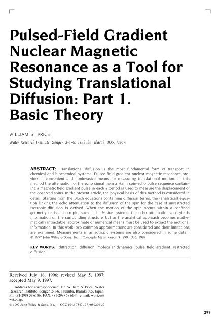
Pulsed-field gradient nuclear magnetic resonance as a tool for ...

Pulsed-Field Gradient 

Nuclear Magnetic 

Resonance as a Tool for 

Studying Translational 

Diffusion: Part 1. 

Basic Theory 

WILLIAM S. PRICE 

Water Research Institute, Sengen 2-1-6, Tsukuba, Ibaraki 305, Japan 

ABSTRACT: Translational diffusion is the most fundamental form of transport in 

chemical and biochemical systems. Pulsed-field gradient nuclear magnetic resonance provides 

a convenient and noninvasive means for measuring translational motion. In this 

method the attenuation of the echo signal from a Hahn spin-echo pulse sequence containing 

a magnetic field gradient pulse in each period is used to measure the displacement of 

the observed spins. In the present article, the physical basis of this method is considered in 

detail. Starting from the Bloch equations containing diffusion terms, the ( analytical) equation 

linking the echo attenuation to the diffusion of the spin for the case of unrestricted 

isotropic diffusion is derived. When the motion of the spin occurs within a confined 

geometry or is anisotropic, such as in in vivo systems, the echo attenuation also yields 

information on the surrounding structure, but as the analytical approach becomes mathematically 

intractable, approximate or numerical means must be used to extract the motional 

information. In this work, two common approximations are considered and their limitations 

are examined. Measurements in anisotropic systems are also considered in some detail. 

1997 John Wiley & Sons, Inc. Concepts Magn Reson 9: 299 336, 1997 

KEY WORDS: diffraction, diffusion, molecular dynamics, pulse field gradient, restricted 

diffusion 

Received July 18, 1996; revised May 5, 1997; 

accepted May 9, 1997. 

Address for correspondence: Dr. William S. Price, Water 

Research Institute, Sengen 2-1-6, Tsukuba, Ibaraki 305, Japan. 

Ph: Ž 81-298. 58 6186, FAX: Ž 81-298. 58 6144. e-mail: wprice@ 

wri.co.jp. 

1997 John Wiley & Sons, Inc. CCC 1043-734797050299-37 

299

300 

PRICE 

INTRODUCTION 

Self-diffusion is the random translational motion 

of molecules Ž or ions. driven by internal kinetic 

energy. Translational diffusion Žnot 

to be confused 

with spin diffusion or rotational diffusion. 

is the most fundamental form of transport Ž 13. 

and is responsible for all chemical reactions, since 

the reacting species must collide before they can 

react Ž 4 . . Diffusion is also closely related to 

molecular size, as can be seen from the Stokes 

Einstein equation, 

kT 

D 1 f 

where k is the Boltzmann constant, T is temperature, 

and f is the friction coefficient. For the 

simple case of a spherical particle with an effective 

hydrodynamic radius Ž i.e., Stokes radius. rS in 

a solution of viscosity the friction factor is given 

by 

 

f6r . 2 

S 

Generally, however, molecular shapes are more 

complicated and may include contributions from 

factors such as hydration, and the friction factor 

must be modified accordingly Ž 49 . . As a consequence, 

the diffusion also provides information 

on the interactions and shape of the diffusing 

molecule. 

Because of its noninvasive nature, nuclear 

magnetic resonance Ž NMR. spectroscopy is a 

unique tool for studying molecular dynamics in 

chemical and biological systems Ž 1019 . . There 

are two main ways in which NMR may be used to 

study self-diffusion coefficients, which are also 

known as tracer-diffusion or intradiffusion coefficients 

Ž 11, 13, 20. Ž Fig. 1 . : Ž a. analysis of relaxation 

data e.g., Refs. Ž 21, 22. and Ž b. pulsed-field 

gradient Ž PFG. NMR. However, the two methods 

report on motions in very different time scales 

and thus, even though a translational diffusion 

coefficient can be derived in both cases, the two 

estimates will agree only under certain circumstances 

Ž 23. since the relaxation method is in fact 

sensitive to rotational diffusion, whereas the PFG 

method measures translational diffusion. Generally, 

in experiments involving the solution state, 

relaxation measurements are sensitive to motions 

occurring in the picosecond to nanosecond time 

scalethat is, motion on the time scale of the 

reorientational correlation of the nucleus. While 

in PFG measurements, motion is measured over 

the millisecond to second time scale. 

In the first method, relaxation data are analyzed 

to determine the rotational correlation 

timeŽ.Ž s . of a probe species Ž 24 . . can then 

c c 

be related to the solution viscosity, and ulti- 

mately, to the translational diffusion coefficient 

Ž . Ž . 

Fig. 1 by using the Debye equation 2527 , 

3 Ž . 

4r 3kT 3 

c S 

and the StokesEinstein equation Ži.e., Eq. . 1 . 

However, a number of assumptions which, depending 

upon the system being studied, may or 

may not be justified need to be made in performing 

this analysis. First, the relaxation mechanism 

of the probe species needs to be known, and it is 

required that the intermolecular contributions to 

the relaxation can be separated from the intramolecular 

contributions Ž 28 . . Second, only if 

the molecule is spherical can its rotational dynamics 

be properly characterized by a single correlation 

time. Third, depending on the size of the 

probe molecules compared to the molecules of 

the bulk solution, they may not see the solution 

as being continuous; as a consequence, one of the 

basic requirements for the validity of the Debye 

equation is violated Ž 8, 9 . . Thus, serious assumptions 

are involved in applying this method to 

studying biological systems when a small probe 

species is used since the solution normally has a 

large macromolecular component Že.g., 

a large 

part of the cytoplasm of red blood cells is composed 

of hemoglobin . . The final problem with this 

method is that the Stokes radius of the probe 

molecule needs to be known and the determination 

of this is not straightforward. 

In the PFG method, the attenuation of a spinecho 

signal resulting from the dephasing of the 

nuclear spins due to the combination of the translational 

motion of the spins and the imposition of 

spatially well-defined gradient pulses is used to 

measure motion. In contradistinction to the relaxation 

method, no assumptions need to be made 

regarding the relaxation mechanismŽ. s or in relat- 

ing to the translational motion of the probe 

c 

molecule. However, to determine the ‘‘true’’ diffusion 

coefficient, D, as against an ‘‘apparent’’ 

diffusion coefficient D the effects of structural 

app 

boundaries that affect the natural diffusion of the 

probe species need to be considered. The mathematics 

required to model anything except for free 

diffusion or diffusion within simple geometries 

becomes rather complicated, and as a result, ana-

PULSED-FIELD GRADIENT NMR 301 

Figure 1 Schematic representation of the relaxation and pulsed-field gradient methods for 

determining molecular dynamics. In our representation of the relaxation method, we have 

assumed that the probe molecule is a sphere with an effective hydrodynamic radius of r . 

S 

lytical solutions are generally not possible and 

numerical solutions must be sought. 

In practice, both B Ž i.e., magnetic. 0 and B1 

i.e., radiofrequency Ž rf. gradients Ž 15, 29, 30. can 

be used, but in the present article we will concentrate 

on B0 gradients, although it should be noted 

that the theoretical aspects are generally analogous. 

The application of B0 gradients to highresolution 

NMR is now commonplace and provides 

superior methods of water suppression, 

coherence selection, and quadrature detection, 

and methods for controlling the effects of radia- 

tion damping Ž 15, 19, 3140 . . Gradients also provide 

the basis of spatial resolution in NMR microscopy 

and imaging i.e., 

magnetic resonance 

imaging Ž MRI. Ž 4144 . , but the application of 

B0 gradients to the study of molecular dynamics is 

less widespread. Gradients afford a powerful tool 

not only for studying molecular diffusion Žunder 

17 2 1 favorable circumstances down to 10 m s . , 

but also for providing structural information in 

the range of 0.1100 m when the diffusion is 

restricted Ž e.g., diffusion in a cell. on the NMR 

time scale. The use of magnetic field gradients

302 

PRICE 

allows diffusion to be added to the standard NMR 

observables of chemical shifts and relaxation times 

Ži.e., longitudinal or T 1; transverse or T 2; 

and in 

the rotating frame or T . 1 . Gradient-based diffusion 

measurements have been found to have clinical 

utility in NMR imaging studies Ž 4549. especially 

in regard to study of cerebral ischaemia 

e.g., Ref. Ž 50. and references therein . 

The aim of this article is to present an introduction 

to the PFG experiment and the theoretical 

basis used for interpreting the data, to determine 

the diffusion coefficient of a probe species 

and perhaps information on the geometry in which 

it is diffusing. As it is not possible to provide a 

comprehensive review of the literature in a single 

paper, a number of pertinent references have 

been mentioned in the text that may be consulted 

for more in-depth coverage of some aspects. The 

analysis of PFG NMR experiments is inherently 

mathematical, and general books on mathematical 

methods e.g., Ref. Ž 51 ., 

mathematical functions 

e.g., Ref. Ž 52 ., and integrals e.g., 

Ref. 

Ž 53. are useful references. Particular emphasis is 

placed on developing a physical feeling for the 

PFG method. It should be noted that the theory 

presented is quite general and applies equally to 

both in io and in itro samples. In the next 

section, the effects of a magnetic gradient on 

nuclear spins is discussed, followed by an intuitive 

explanation of how diffusion can be related to the 

attenuation of the echo signal in the PFG NMR 

experiment. Finally, the concept of restricted diffusion 

is introduced. In the third section, the 

mathematical background relating diffusion to the 

echo attenuation and the experimental parameters 

is considered in detail. First, an analytical 

macroscopic approach starting from the Bloch 

equation is derived. The effects of flow superimposed 

upon diffusion are also considered. Next, 

two common approximate methods, the Gaussian 

phase distribution Ž GPD. approximation and the 

short gradient pulse Ž SGP. approximation, are 

presented. To illustrate these approaches, equations 

relating echo attenuation to the experimental 

variables and the diffusion coefficient are derived 

for the case of free diffusion. The analogy 

between PFG measurements and scattering is explained. 

Finally, the concepts of ‘‘diffusive 

diffraction’’ and of imaging molecular motion are 

illustrated using diffusion within a rectangular 

barrier pore as an example. In the final section, 

we consider the general relationships between the 

experimental variables and echo attenuation in 

restricted geometries and the validity of the GPD 

and SGP approximations. The differences and 

similarities between the two approaches are elucidated 

pictorially using the example of diffusion in 

a sphere. PFG diffusion measurements in anisotropic 

systems, which commonly occur in liquid 

crystal and in io studies, are examined in the 

last subsection of the article. 

NUCLEAR SPINS, GRADIENTS, AND 

DIFFUSION 

Magnetic Gradients as Spatial Labels 

All of the NMR theory needed for understanding 

the effects of B0 gradients on nuclear spins has 

the Larmor equation as the origin: 

 

B 4 

0 0 

Ž 

1 where is the Larmor frequency radians s . 

0 

, 

Ž 1 1 is the gyromagnetic ratio rad T s . , B Ž T. 0 is 

the strength of the static magnetic field, and we 

have neglected the small effect of the shielding 

constant. We consider B0 to be oriented in the 

z-direction. Since B0 is spatially homogeneous, 

is the same throughout the sample. Equation 4 

holds for a single quantum coherence Ž i.e., n 1. . 

However, if in addition to B0 there is a spatially 

Ž 1 dependent magnetic field gradient g Tm . , 

and accounting for the possibility of more than 

single quantum coherence, becomes spatially 

dependent, 

Ž . Ž Ž .. 

n,r n gr 5 

eff 0 

where we define g by the grad of the gradient 

field component parallel to B , i.e., 

0 

B z B z B z 

gB i j k 6 0 

x y z 

where i, j, and k are unit vectors of the laboratory 

frame of reference. The important point is that if 

a homogeneous gradient of known magnitude is 

imposed throughout the sample, the Larmor frequency 

becomes a spatial label with respect to the 

direction of the gradient. In imaging systems, 

which typically can produce equally strong magnetic 

field gradients in each of the x, y, and z 

directions, it is possible to measure diffusion along 

any of the x, y, orz-directions Žor 

combinations 

thereof . ; however, in normal NMR spectrometers, 

it is more common to measure diffusion with

the gradient oriented along the z-axis Ži.e., 

parallel 

to B . 0 . For simplicity, in most of the present 

article we are concerned only with the case where 

the gradient is oriented along z, although some 

attention is paid to the use of gradients along 

more than one axis when we consider anisotropic 

diffusion in the final subsection. In the case of a 

single gradient oriented along z, the magnitude 

of g is only a function of the position on the 

z-axis, g z g k, which we will henceforth refer 

to simply as g. It can be seen from Eq. 5 that 

successively higher Ž homonuclear. quantum transitions 

are more sensitive to the effects of the 

gradient, whereas zero quantum transitions are 

unaffected by the presence of the gradient. For 

heteronuclear multiple quantum transitions, Eq. 

5 must be modified to account for the coherent 

spins. 

In the case of a single quantum coherence, we 

can see from Eq. 5 that for a single spin the 

cumulative phase shift is given by 

H 

t 

0 0 

static field 

applied gradient 

Ž t. Bt gŽ t. zŽ t. dt 7 

where the first term on the right-hand side corresponds 

to the phase shift due to the static field, 

and the second term represents the phase shift 

due to the effects of the gradient. Thus, from the 

second term of Eq. 7 we can see that the degree 

of dephasing due to the gradient pulse is proportional 

to the type of nucleus Ž i.e., . , the strength 

of the gradient Ž i.e., g . , the duration of the gradient 

Ž i.e., t . , and the displacement of the spin 

along the direction of the gradient. Although the 

gradient is normally applied in a pulse of constant 

amplitude, we have written g as gt Ž. in Eq. 7 to 

emphasize that the gradient may itself be a function 

of time Ž i.e., not merely a rectangular pulse . . 

However, for simplicity, in the present article we 

will concern ourselves only with constant amplitude 

pulses. In this case we can think of the 

‘‘area’’ or ‘‘dephasing strength’’ of the gradient 

pulse as equaling gt. 

Measuring Diffusion with Magnetic Field 

Gradients 

Ž . 

From Eq. 5 it is apparent that a well-defined 

magnetic field gradient can be used to label the 

position of a spin, albeit indirectly, through the 

Larmor frequency. This provides the basis for 


measuring diffusion. The most common approach 

is to use a simple modification Ž 5456. of the 

Hahn spin-echo pulse sequence Ž 5759 . , in which 

equal rectangular gradient pulses of duration 

are inserted into each period Žthe 

‘‘Stejskal and 

Tanner sequence’’ or ‘‘PFG sequence’’ .Ž Fig. 2 . . 

Applying the magnetic field gradient in pulses 

instead of continuously i.e., 

steady gradient experiment 

Ž 57, 58. circumvents a number of experimental 

limitations Ž 54 . : Ž a. Since the gradient 

is off during acquisition, the line width is not 

broadened by the gradient, and thus the method 

is suitable for measuring the diffusion coefficient 

of more than one species simultaneously. Ž b. The 

rf power does not have to be increased to cope 

with a gradient-broadened spectrum. Ž. c Smaller 

diffusion coefficients can be measured since it is 

possible to use larger gradients. Ž d. The time over 

which diffusion is measured is well defined because 

the gradient is applied in pulses; this is of 

particular importance to studies of restricted diffusion 

Ž see the next section . . Ž e. As the gradient 

is applied in pulses it is Ž normally. possible to 

separate the effects of diffusion from spinspin 

relaxation; this will be explained below. Generally, 

the applied gradient pulses are much stronger 

than any background gradients that may be present; 

as a result, the background gradients Že.g., 

due to differences in susceptibility in the sample, 

inhomogeneities in the main magnetic field, etc. . 

will be neglected in the analysis given below. 

We will now qualitatively explain how this 

method works. The mechanism is shown schematically 

in Fig. 2. Imagine that we have an ensemble 

of diffusing spins at thermal equilibrium Ži.e., 

the 

net magnetization is oriented along the z-axis . . A 

2 rf pulse is applied which rotates the macroscopic 

magnetization from the z-axis into the xy 

plane Ž i.e., perpendicular to the static field . . During 

the first period at time t 1, 

a gradient pulse 

of duration and magnitude g is applied so that 

at the end of the first period, spin i experiences 

a phase shift, 

i 0 

static field 

t1 t 1 

i 

applied gradient 

Ž . B g z Ž t. dt 8 H 

 

where the first term is the phase shift due to the 

main field, and the second one due to the gradient. 

Different from Eq. 7 we have taken g out 

of the integral in Eq. 8 since we are considering 

a constant amplitude gradient.

304 

PRICE 

At the end of the first period, a rf pulse is 

applied that has the effect of reversing the sign of 

the precession Ž i.e., the sign of the phase angle. 

or, equivalently, the sign of the applied gradients 

and static field. At time t1 , a second gradient 

pulse of equal magnitude and duration is applied 

Žn.b., the pulse has the effect of changing the 

sign of the first gradient pulse; this leads to the 

idea of an ‘‘effective’’ field gradient; see The 

Macroscopic Approach . . If the spins have not 

undergone any translational motion with respect 

to the z-axis, the effects of the two applied gradi-

ent pulses cancel and all spins refocus. However, 

if the spins have moved, the degree of dephasing 

due to the applied gradient is proportional to the 

displacement in the direction of the gradient Ži.e., 

the z-direction. in the period Ži.e., 

the duration 

between the leading edges of the gradient pulses . . 

Thus, at the end of the echo sequence, the total 

phase shift of spin i relative to being located at 

z 0 is given by 

½ H 5 

i 

 

0 

t1 t1 

i 

 

first period 

t1 B g z Ž t. ½ 0 H 

i dt5 

t1 

second period 

t1t1 g z Ž t. dt z Ž t. ½H i H 

i dt5 

t1 t1 Ž 2. B g z Ž t. dt 

 

9 

We should recall that in NMR we are concerned 

Ž 

with an ensemble of nuclei with different spatial 


starting and finishing positions . , and thus, the 

normalized intensity Ž i.e., an attenuation. of the 

echo signal at t 2 

Ž 58, 60 . , 

i.e., SŽ 2. is given by 

H 

 

Ž . Ž . Ž . i 

g0 

 

S 2 S 2 P ,2 e d. 10 

where SŽ 2. is the signal Ž 

g0 

i.e., resultant mag- 

netic moment. in the absence of a field gradient. 

If we consider only the real component of SŽ 2 . , 

and recalling De Moivre’s theorem, 

we have 

i 

e cos i sin 11 

H 

 

SŽ 2. SŽ 2. PŽ ,2. cos d 12 g0 

where PŽ ,2. is the Ž relative. phase-distribution 

function. For the PFG sequence, some authors 

write PŽ , . , since it is the gradient pulses and 

the separation between them that constitute the 

Figure 2 A schematic representation of how the Stejskal and Tanner Ž or PFG. pulse 

sequence measures diffusion and flow. This is a Hahn spin-echo pulse sequence with a 

rectangular gradient pulse of duration and magnitude g inserted into each delay. The 

separation between the leading edges of the gradient pulses is denoted by . The applied 

gradient is generally along the z-axis Ž the direction of the static field . . The second half of the 

echo is digitized Ž denoted by dots. and used as the free induction decay Ž FID . . In this 

schematic description, we assume that we start the pulse sequence with a sample consisting 

of four in-phase spins Ž really an ensemble! . and we consider only the precession due to the 

gradient Ž i.e., we use a rotating reference frame rotating at . 0 . We assume that the center 

of the gradient coincides with the center of the sample Ž i.e., z 0 . . Accordingly, the spins 

above and below this point acquire phase shifts owing to the gradient pulses, but in opposite 

senses. In the absence of diffusion, the effect of the first gradient pulse, denoted by the 

curved arrows in the first phase diagram, is to create a magnetization helix Ži.e., 

the solid 

ellipses in the center phase diagram. with a pitch of 2 Ž g . . Although we have 

represented the gradient pulses as having a finite width it is easier to consider them in the 

limit of 0 Ž i.e., the short gradient pulse limit . . The pulse reverses the sign of the 

phase angle Ž i.e., the dotted ellipses in the center phase diagram . , and thus, after the second 

gradient pulse, the helix is unwound and all spins are in phase, which gives a maximum echo 

signal. In the presence of diffusion, the winding and unwinding of the helix are scrambled by 

the diffusion process, resulting in a distribution of phases, although it is not easily seen since 

our sample consists of only four spins. Larger diffusion would be reflected by poorer 

refocusing of the spins, and consequently by a smaller echo signal. The effects of restriction 

upon the diffusion process will also contribute to this loss of phase coherence. In the 

absence of any background gradients, diffusion in the periods before Ž e.g., 0 t . 1 and after 

Ž i.e., t . 1 the gradient pulses does not affect the signal attenuation. In the presence 

of flow Ž imagine that the outflowing spins are replaced by inflowing spins. along the 

direction of the gradient Ž in the z direction with velocity in the present example. and 

neglecting diffusion, all the spins receive the same change in phase. The greater the flow is, 

the larger is the net phase change. If both diffusion and flow processes are present, then the 

whole diffusion-induced phase distribution receives a net phase shift.

306 

PRICE 

‘‘active’’ part of the sequence. By definition, 

Ž . 

P ,2 must be a normalized function, and so 

 

H 

 

Ž . 

P ,2 d1. 13 

Below, we will consider the further derivation 

of Eq. 12 in the context of the GPD approximation 

Ž see The GPD Approximation . . However, for 

the present, Eqs. 9 and 12 provide a very clear 

conceptual idea as to how the PFG method works. 

From Eq. 9 , it can be seen that the phase shift 

due to the static field cancels. In the absence of 

diffusion, the phase shifts due to the two gradient 

pulses Žor, 

conversely, in the presence of diffusion 

but with g 0. will also cancel; thus, i 0 for 

all i, and as cos 1 in Eq. 12 , 

a maximum 

signal will be recorded Žsee 

the first series of 

phase diagrams in Fig. 2 . . However, if we have 

diffusion, then the displacement function z Ž. i t is 

time dependent and the phase shifts accumulated 

by an individual nucleus due to the action of the 

gradient pulses in the first and second periods 

Žduring the gradient pulses to be precise see Eq. 

9 ; n.b., we neglect the effects of background 

gradients. do not cancel. The degree of miscancellation 

Ž i.e., larger phase shift. increases with 

increasing displacement due to diffusion Ži.e., 

random 

motion. along the gradient axis. These random 

phase shifts resulting from the diffusion are 

averaged over the whole ensemble of nuclei that 

contribute to the NMR signal. Hence, the observed 

NMR signal is not phase shifted but attenuated, 

and the greater the diffusion is, the larger 

is the attenuation of the echo signal Žsee 

the 

second series of phase diagrams in Fig. 2 . . Simi- 

larly, as the gradient strength is increased in the 

presence of diffusion the echo signal attenuates. 

In Fig. 3 some experimental 13 C-NMR PFG spec- 

tra of 13 CCl are presented to illustrate the loss 

4 

of echo signal intensity due to diffusion. Net flow, 

on the other hand, causes a net phase shift of the 

echo signal Žsee 

the third series of phase diagrams 

in Fig. 2 and the end of this subsection. 

instead of the diffusion-induced ‘‘blurring’’ of the 

phases which results in a diminution of the echo 

signal. 

It is important to understand the difference 

between gradient echoes and spin echoes. In 

measuring diffusion, we generally choose to use 

the PFG pulse sequence Ži.e., 

a spin-echo sequence. 

instead of a gradient-echo pulse sequence 

Ži.e., 

the PFG pulse sequence without the 

pulse and with the second gradient pulse having 

an opposite polarity to the first pulse . . The 

reason is that as well as refocusing the sign of the 

phase angle accumulated during the first period, 

the pulse has the effect of refocusing 

chemical shifts and the frequency dispersion due 

to the residual B0 inhomogeneity and susceptibility 

effects in heterogeneous samples, etc. A gradi- 

Figure 3 13 C-PFG NMR spectra of a sample of 13 CCl . The spectra were acquired at 303 K 

4 

with 100 ms, 4 ms, and g ranging from 0 to 0.45 T m 1 in 0.05-T m 1 increments. 

The spectra are presented in phase-sensitive mode with a line broadening of 5 Hz. As the 

intensity of the gradient increases, the echo intensity decreases due to the effects of 

diffusion.

ent echo, on the other hand, refocuses only the 

phase dispersion resulting from the gradient 

pulses. It is because of the additional properties 

of spin echoes that diffusion measurements are 

almost invariably performed using spin-echo 

based sequences. 

In our discussion above, we did not consider 

the relaxation process that occurs during the echo 

sequence. Thus, in the absence of diffusion 

andor the absence of gradients, we would have 

the signal at t 2 equal to 

2 

SŽ 2. SŽ 0. exp 14 g0 ž 

T / 2 

where SŽ. 0 is the signal without attenuation due 

to relaxationthat is, the signal that would be 

observed immediately after the 2 pulse. We 

assume here that the observed signal originates 

from a single species Ži.e., 

the observed signal 

results from one population with a single relaxation 

time . . In the presence of diffusion and 

gradient pulses, the attenuation due to relaxation 

and the attenuation due to diffusion and the 

applied gradient pulses are independent, and so 

we can write, 

ž T / 2 

attenuation due to 

2 

SŽ 2. SŽ 0. exp f Ž , g , , D. 

attenuation due to 

relaxation 

diffusion 

 

15 

where fŽ , g, , D. is a function that represents 

the attenuation due to diffusion Že.g., 

compare 

Eq. 15 with Eq. 10 . . Thus, if the PFG measurement 

is performed whilst keeping constant, it is 

possible to separate the contributions. Hence, by 

dividing Eq. 15 by Eq. 14 we normalize out the 

attenuation due to relaxation, leaving only the 

attenuation due to diffusion, 

SŽ 2. 

E fŽ , g,, D . . 16 SŽ 2. g0 

In the steady-gradient experiment Ži.e, 

 

. , however, since the gradients are on for all of 

the sequence, only g can be altered independently 

of . Recall the well-known diffusion term 

in the expression for the intensity of the Hahn 


Ž . 

spin-echo sequence 5759 , 

Ž . Ž . Ž . Ž 2 2 3 S 2 S 0 exp 2T exp 2 Dg 3 . , 

2 

 

attenuation due 

to relaxation 

attenuation due 

to diffusion 

 

17 

whereas in the PFG experiment, we can alter , 

, orgindependently of and still perform this 

normalization. This is a very important distinction 

between the steady-gradient diffusion experiment 

and the PFG experiment. 

Although the effects of relaxation are normalized 

out, since we use E as our experimental 

measure, the time scale of the experiment Ž i.e, . 

is limited by the relaxation time of the probe 

species. As increases, so must , and eventually 

the signal will become too small to measure Žsee 

Eq. 14 . . The smallest value of will be limited 

by the performance of the gradient system. In 

practice, is normally between 1 ms and 1 s. 

must be smaller than and is typically in the 

range of 010 ms. The magnitude of g is machine 

dependent, and currently the largest gradient 

pulses on commercially available equipment are 

of the order of 20 T m1 . 

We now need to equate the attenuation Ž E. of 

the echo signal to the experimental variables; that 

is, we need to derive fŽ , g, , D . . The methods 

for doing this will be presented in the next section. 

However, we first need to digress a little and 

consider diffusion itself. 

Free and Restricted Diffusion 

In the PFG experiment, we probe the particle’s 

motion by taking a measurement at time t t1 and a second measurement at time t t1 . 

The key point is that in the PFG experiment the 

echo attenuation gives information on the displacement 

along the gradient axis Žthe 

z-axis in 

the present case. that has occurred during the 

period , which can then be related to the diffusion 

coefficient but it does not, at least directly, 

give us information on how the particle moved 

between the initial and the final positions. Specifically, 

it gives information on the self-correlation 

function Ž 61 . , PŽ r , r , t. 0 1 that is, the conditional 

probability of finding a particle initially at a position 

r , at a position r after a time t. PŽ r , r , t. 

0 1 0 1 

is given by the solution of the diffusion equation. 

Hence we need to examine the diffusion equation 

and how we can obtain PŽ r , r , t. from it. 

0 1

308 

PRICE 

In terms of the concentration in number of 

particles per unit volume, cŽ r, t . , the flux of a 

particle is given by Fick’s first law of diffusion to 

be for example, see Ref. Ž 2, 62 ., 

Ž . Ž . 

Jr,t Dc r,t . 18 

Ž . 

The minus sign indicates that in isotropic media 

the direction of flow is from larger to smaller 

concentration. Because of the conservation of 

mass, the continuity theorem applies, and thus, 

Ž . 

c r,t 

t 

Ž . 

Jr,t . 19 

In other words, Eq. 19 states that cŽ r, t. t is 

the difference between the influx and efflux from 

the point located at r. Combining Eqs. 18 and 

19 we arrive at Fick’s second law of diffusion 

e.g., Refs. Ž 4, 51, 62 ., 

Ž . 

c r,t 

t 

2 Ž . 

D c r,t 20 

So far in our mathematical descriptions of 

diffusion, we have, perhaps simplistically, assumed 

that the diffusion process is isotropic and 

can therefore be described by the isotropic diffusion 

coefficient D Ž i.e., a scalar . . More generally 

the diffusion process is represented by a cartesian, 

or rank two, tensor Ž i.e., a 3 3 matrix. 

Ž 51 . , D ŽD 

where and take each of the 

Cartesian directions . ; thus, written more generally, 

Eq. 18 can be written as 

which is shorthand for 

Ž . Ž . 

Jr,t Dc r,t , 21 

Ž . 

c x,t 

D D D 

x 

JŽ x,t. xx xy xz 

cŽ y,t. 

JŽ y,t. Dyx DyyDyz . 

y 

JŽ z,t. Dzx Dzy Dzz 

cŽ z,t. 

z 

 

22 

We note that the diagonal elements of D, Že.g., 

. scale concentration gradients and fluxes 

in the same direction, the off-diagonal elements 

Ž e.g., . couple fluxes and concentration gra- 

dients in orthogonal directions, and similarly, Eq. 

 

20 becomes 

Ž . 

c r,t 

t 

Ž . 

Dc r,t . 23 

For simplicity in most of what follows, we are 

concerned only with isotropic diffusion. However, 

in the section on anisotropic diffusion, we will 

consider in detail the significance of anisotropic 

diffusion in PFG diffusion measurements. 

In the case of self-diffusion, there is no net 

concentration gradient, and instead we are concerned 

with the total probability, PŽ r , t. 1 of finding 

a particle at position r1 at time t. This is given 

by 

H 

PŽ r ,t. Ž r . PŽ r ,r ,t. dr 24 1 0 0 1 0 

where Ž r . is the particle density Ž 

0 

the formal 

definition of the particle density is considered in 

detail below . , and thus, Ž r . PŽ r , r , t. 0 0 1 is the 

probability of starting from r 0 and moving to r1 in 

time t. The integration over r 0 accounts for all 

possible starting positions. Similar to concentration, 

PŽ r , t. 1 describes the probability of finding 

a particle in a certain place at a certain time. 

PŽ r ,t. 1 is a sort of ensemble-averaged probability 

concentration for a single particle, and it is thus 

reasonable to assume that it obeys the diffusion 

equation Ž 41 . . Because the spatial derivatives in 

Fick’s laws refer to r 1, 

we can rewrite Fick’s laws 

in terms of PŽ r , r , t. with the initial condition, 

0 1 

Ž . Ž . 

P r ,r ,0 r r 25 

0 1 1 0 

Žn.b., in Eq. 25 is the Dirac delta function, not 

the length of the gradient pulse . . Thus, if in Eq. 

18 PŽ r , r , t. is substituted for cŽ r, t . 

0 1 

, J becomes 

the conditional probability flux. Similarly, 

in terms of PŽ r , r , t. Eq. 20 becomes 

0 1 

PŽ r ,r ,t. 

0 1 2 D PŽ r ,r ,t . . 26 0 1 

t 

In the case of anisotropic diffusion, Eq. 26 can 

be changed similarly to Eq. 23 . PŽ r , r , t. 0 1 is 

commonly termed the Green’s function or diffusion 

propagator Ž 55, 63 . .

For the case of Ž three-dimensional. diffusion 

in an isotropic and homogeneous medium Ži.e., 

boundary condition P 0asr ,P . Ž r ,r ,t. 

1 0 1 

can determined from Eq. 26 using Fourier transforms 

Ž 64. and is given by Ž 62. 

32 

2 

Ž r r . 1 0 

4Dt / 

PŽ r ,r ,t. Ž 4Dt. exp . 

0 1 ž 

27 Equation 27 states that the radial distribution 

function of the spins in an infinitely large system 

with regard to an arbitrary reference time is 

Gaussian. We note from Eq. 27 that PŽ r , r , t. 

0 1 

does not depend on the initial position, r , but 

0 

depends only on the net displacement, r r 

1 0 

Žthe vector r r moved during time t is often 

1 0 

referred to as the dynamic displacement R . . This 

reflects the Markovian nature Ž 10, 65. of Brownian 

motion. The solution of Eq. 26 becomes 

much more complicated when the displacement 

of the particle is affected by its boundaries Že.g., 

diffusion in a sphere. and PŽ r , r , t. 0 1 is no longer 

Gaussian. The solutions of Eq. 26 for many 

cases of interest can be found in the literature 

Ž 62, 66 . . It should be noted that the mathematics 

of heat conduction, after making the appropriate 

changes of notation, is identical to that for describing 

diffusion Ž 62 . . 

It is an appropriate stage to consider the Ž r . 0 , 

the probability that a spin starts at r 0, 

in some 

detail. Formally, Ž r . is given by 

H 

0 

Ž r . lim P Ž r , r , t. dr 28 0 0 1 1 

t 

and thus is independent of r 0, 

because after infinite 

time the finishing position of a particle in the 

system will be independent of the starting position. 

PŽ r , r , t. as given by Eq. 27 Ž 

0 1 

i.e., free 

diffusion. approaches 0 as t , but the ‘‘effective 

volume’’ Ž i.e., the integral over r . 1 becomes 

proportionally larger; consequently, Ž r . 0 stays 

constant Ž 1 is a convenient choice . . In the case of 

an enclosed geometry, Ž r . 0 is given by the inverse 

of the volume. Also, by definition we must 

have e.g., ref. Ž 65. 

Ž . 

r dr 1. 29 

H 0 0 


The mean-squared displacement is given by 

Ž . 

e.g., Ref. 10 

2 ² Ž r r . 1 0 : 

 

2 

H Ž . Ž . Ž . 

1 0 0 0 1 0 1 

 

r r r P r ,r ,t dr dr . 

 

30 

Using PŽ r , r , t. as given by Eq. 27 

0 1 

, we can 

calculate the mean-squared displacement of free 

diffusion. To do this we rewrite Eq. 27 in Cartesian 

form Ž i.e., r xi y j zk. 

PŽ r ,r ,t. Ž 4Dt. exp 

0 1 ž 

exp 

32 

2 

Ž x x . 1 0 

4Dt / 

ž 

2 

Ž y y . 1 0 

4Dt / 

ž 

2 

Ž z z . 1 0 

4Dt / 

exp 31 and using Eq. 30 and noting that Ž r . 0 1 for 

the case of free diffusion. We can evaluate Eq. 

30 using the standard integral e.g., 

Eq. 3.462 8. 

in Ref. Ž 53 ., 

H 

2 2 x 2 x 

x e dx 

( ž / 

2 

1 2 

12 e 

2 

 

arg ,Re0 32 

where in our case x x1x 0, y1y 0, z1z 0, 

Ž . 1 4Dt and 0, and thus we obtain Žn.b. 

for free diffusion. 

2 ² 1 0 : 

Ž r r . nDt 33 where n 2, 4, or 6 for one, two, or three dimensions, 

respectively. Equation 30 presents a relationship 

between the molecular displacement due 

to diffusion and the diffusion equation. Specifically 

for free diffusion, it states that the meansquared 

displacement changes linearly with time. 

When we use the PFG method to measure 

diffusion in free solution and in the absence of 

exchange, the length of time we choose Ž i.e., . is 

irrelevant and we get the same result Ži.e., 

from 

Eq. 33 the mean-squared displacement scales 

linearly with time . . This is, of course, assuming 

that the relaxation timeŽ. s of the species in ques-

310 

PRICE 

tion is sufficiently long so that we still get a 

measurable signal and that the measurement is 

unaffected by eddy currents or other experimental 

complications see, for example, ref. Ž 19 .. 

However, in the case of a species diffusing within 

a confined space we must be careful to properly 

account for the effects of the restricting geometry 

on the motion of the species. If a particle is 

diffusing within a restricted geometry Žsometimes 

referred to as a ‘‘pore’’ . , the displacement along 

the z-axis will be a function of , the diffusion 

coefficient, and the size and shape of the restricting 

geometry. Consequently, if the boundary effects 

are not properly accounted for and we analyze 

the data using the model for free diffusion 

Ž see the next section . , we will measure an apparent 

diffusion coefficient Ž D . app and not the true 

diffusion coefficient. We illustrate this effect later 

in this section. 

Before further considering the problem of restricted 

diffusion, it is appropriate to briefly consider 

what constitutes the true diffusion coefficient. 

In a pure liquid Ž e.g., water. the true diffusion 

coefficient corresponds to the bulk diffusion 

coefficient. However, the situation is rather more 

complex in a macromolecular solution Že.g., 

cell 

cytoplasm, polymer solutions, protein solutions, 

etc. . where the probe molecule Ž e.g., water. has to 

skirt around the larger ‘‘obstructing’’ molecules 

Ž e.g., proteins, organelles. as well as perhaps interacting 

with protein hydration shells e.g., 

Ref. 

Ž 67 .. 

These effects operate on a time scale much 

smaller than the smallest experimentally available 

and consequently are well averaged on the time 

scale of . For example, if we consider a reasonably 

small value of of 5 ms and that at 298 K 

water has a diffusion coefficient of about 2.3 

9 2 1 Ž . 

10 m s 68, 69 , then from Eq. 30 the mean 

displacement of a water molecule during is 

about 5 m. The true diffusion coefficient will be 

an average bulk diffusion coefficient consisting of 

all of the interactions that affect the probe 

molecule diffusion. The situation can be further 

complicated by the effects of exchange through 

cell membranes Ž 70 . . The different time scales of 

the averaging processes is one of the major reasons 

that diffusion probed by using relaxation 

studies and diffusion measured using PFG NMR 

are essentially different things with the relaxation 

based measurements probing motion on the time 

scale of the correlation time of the probe molecule 

and not on the Ž much longer. time scale of 

Ž 21, 71 . . We mention in passing that in a polymer 

solution if the diffusion of the polymer itself is 

studied there can be additional complications owing 

to the entanglement of the polymer molecules 

e.g., Ref Ž 19. and references therein . 

We now explain the concept of restricted diffusion 

and how it relates to PFG NMR diffusion 

measurements. Consider two cases where we have 

a particle with the same diffusion coefficient; in 

one case the particle is freely diffusing Ži.e., 

an 

isotropic homogeneous system . , while in the other 

case it is confined to a reflecting sphere of radius 

R Ž Fig. 4 . . By ‘‘reflecting’’ we mean that the spin 

is neither transported through the boundary nor 

relaxed by the contact with the boundary. From 

Eq. 30 , 

we can define the dimensionless variable 

Ž i.e., n 1, t . , 

2 

DR , 34 

which is useful in characterizing restricted diffusion 

as will be seen below. In the case of freely 

diffusing particles, the diffusion coefficient determined 

will be independent of and the displacement 

measured in the z-direction will reflect the 

true diffusion coefficient, since the mean-squared 

displacement scales linearly with time Žsee 

Eq. 

33 . . However, for the particle confined to the 

sphere, the situation is entirely different. For 

short values of such that the diffusing particle 

has not diffused far enough to feel the effect of 

the boundary Ž i.e., 1 . , the measured diffusion 

coefficient will be the same as that observed 

for the freely diffusing species. As becomes 

finite Ž i.e., 1 . , a certain fraction of the particles 

Ži.e., 

in a real NMR experiment there is an 

ensemble of diffusing species. will feel the effects 

of the boundary and the mean squared displacement 

along the z-axis will not scale linearly with 

; thus, the measured diffusion coefficient Ži.e., 

D . will appear to be Ž observation. app 

time depen- 

dent. At very long , the maximum distance that 

the confined particle can travel is limited by the 

boundaries, and thus the measured mean-squared 

displacement and diffusion coefficient becomes 

independent of . Thus, for short values of the 

measured displacement of a particle in a restricting 

geometry observed via the signal attenuation 

in the PFG experiment is sensitive to the diffusion 

of the particle. At long the signal attenuation 

becomes sensitive to the shape and dimensions 

of the restricting geometry. The relationships 

between the experimental parameters are 

further examined in the next section. If the restricting 

geometry is spherically symmetric, then 

there will be no-orientational dependence with


Figure 4 In the PFG experiment, we use the first gradient pulse to label the starting 

position of the diffusing species and the second gradient pulse, at a time later, to probe its 

finishing position with respect to the gradient direction. The important point is that we do 

not know what happens between these two times. In this diagram we schematically represent 

what happens when we measure the diffusion coefficient of a species when it is undergoing 

free diffusion or restricted diffusion in a sphere of radius R. r0 denotes the starting position 

Ž . , and r denotes the position Ž . 

at a time later. The length of the arrows Ž i.e., R. 

1 

denote the measured displacement in the direction of the gradient which is normally in the z 

direction and is taken to be up the page in the present diagram. We consider three relevant 

Ž. Ž 2 time scales for the measurement of the effects of the restricted diffusion; i DR . 

1Ž the short time limit . ; the particle does not diffuse far enough during to feel the 

effects of restriction. Measurements performed within this time scale lead to the true 

diffusion coefficient Ž i.e., D . . Ž ii. 1; some of the particles feel the effects of restriction 

and the diffusion coefficient measured within this time scale will be apparent Ž i.e., D . app and 

be a function of . The fraction of particles that feel the effects of the boundary will be 

dependent on the surface-to-volume ratio S V. Ž iii. 1 Ž the long time limit . 

geo 

; all 

particles feel the effects of restriction. In this time scale, the displacement of the particle is 

independent of and depends only on R. Thus, restriction causes a Ž measuring-time. -dependent 

diffusion coefficient in which at the displacement is limited by the embedding 

geometry. 

respect to the gradient direction of the measured 

displacement. However, particularly in in io 

systems Ž e.g., muscle cells . , where the restricting 

geometry is normally not spherically symmetric, 

and in liquid crystals where the diffusion can be 

anisotropic, the observed signal attenuation will 

have an orientational dependence. This aspect 

will be considered subsequently. 

We should also mention that ‘‘obstruction’’ can 

be thought of as a type of restricted diffusion. 

The change in the diffusion coefficient due to 

obstruction is a source of information on the 

shape of the obstructing particle, e.g., Refs. 

Ž 7274 . . The mathematical description of obstruction 

effects is very difficult, since the diffusion 

path of the probe molecule can be very

312 

PRICE 

complicated; also the obstructing particles are not 

Ž necessarily. distributed in space in a totally ordered 

or totally random way. 

CORRELATING SIGNAL ATTENUATION 

WITH DIFFUSION 

Introduction 

We will now discuss the mathematical formulations 

necessary to relate the signal attenuation to 

the diffusion coefficient and boundary conditions 

in the PFG experiment. Starting from the Bloch 

equations modified to include the diffusion of 

magnetization Ž 75, 76. it is possible to derive the 

necessary relationships analytically for free diffusion, 

as we shall show below. However, in the 

case of restricted diffusion this macroscopic 

approachbecomes mathematically intractable. 

Thus, in general case one is forced to use different 

approximations to find formulae relating E to 

the diffusion coefficient, boundary, and experimental 

conditions. There are two common approximations, 

namely: the GPD approximation 

and the SGP approximation. However, even using 

these approximations, analytic solutions are generally 

not possible and numerical methods must 

be used. In this section, we will only consider the 

case of free diffusion and describe the macroscopic 

approach and the SGP and GPD approximations 

in this case. It is assumed that the gradient 

pulses are rectangular. Detailed discussion of 

the signal attenuation of spins undergoing restricted 

diffusion will be deferred until later in 

this section. 

The Macroscopic Approach 

Bloch Equations Including the Effects of Diffusion. 

The Bloch equations for the macroscopic nuclear 

magnetization, Mr,t Ž . MxMyM, z includ- 

ing the diffusion of magnetization, are given by 

Ž 75, 76 . , 

Mr,t Ž . 

MxiMyj MBr,t Ž . 

t T2 Ž M M . k 

D M. 35 

T1 z 0 2 

In the case of anisotropic diffusion, the last term 

in Eq. 35 would be replaced by DM.Ifwe 

now take Ž as is usually the case. B to be oriented 

0 

along the z-axis and that this is superposed by a 

gradient g vanishing at the origin which is parallel 

to B Ž 0 we assume that the inhomogeneities caused 

by g are much smaller than B . 0 , and thus we can 

write 

B 0, B 0, 

x y 

Ž . 

B B gr B g xg yg z 36 

z 0 0 x y z 

 

If Eq. 36 is then substituted into Eq. 35 , noting 

that 

MB Ž M B MB. Ž MBM B . y 

y z z y x z x x z 

Ž . 

M B M B 37 

x y y x z 

and defining the Ž complex. transverse magnetization 

as 

mM iM 38 x y 

we obtain 

m 

Ž . 

2 

i0mi gr mmT2D m. 

t 

39 The Stejskal and Tanner Pulse Sequence in the 

Absence of Diffusion. In the absence of diffusion 

Ž i.e., D 0,mrelaxes . 

exponentially with a time 

constant T 2, 

and thus we set 

i 0 tt T 2 

me 40 

where represents the amplitude of the precessing 

magnetization unaffected by the effects of 

relaxation. If we substitute Eq. 40 into 39 , 

we 

obtain 

 

t 

Ž . 2 

igr D . 41 

In the absence of diffusion, Eq. 41 is a first-order 

ordinary differential equation with solution 

Ž . Ž . 

r,t Sexp ir F 42 

where S is a constant and 

t 

H 

0 

FŽ t. gŽ t. dt. 43 Now, if we consider the case of the PFG pulse 

sequence, then during the period from the 2 

pulse to the pulse, we have Ži.e., Eq. 42. Ž . Ž . 

r,t Sexp ir F , 44

and S corresponds to the value of immediately 

after the 2 pulse. After the pulse Žneglect 

ing the phase angle of the pulse, which is of no 

consequence here . , we have 

where 

Ž . Ž Ž .. 

r,t Sexp ir F 2f , 45 

Ž . 

fF . 46 

Thus, from Eq. 45 we can see that the effect of 

the pulse is to set back the phase of by twice 

the amount that it had advanced up until the 

pulse Žsee 

the first series of phase diagrams in 

Fig. 2 . . Equations 44 and 45 can then be combined 

into 

Ž . Ž Ž Ž . .. 

r,t Sexp ir F 2 H t f 47 

where Ht Ž. is the Heaviside step function. We 

note here that Eq. 47 is valid for the Hahn 

spin-echo pulse sequence. 

The Stejskal and Tanner Pulse Sequence in the 

Presence of Diffusion. In the previous section, we 

considered the solution to Eq. 41 in the absence 

of the diffusion. In this section, we derive a 

solution to Eq. 41 including the effects of diffusion. 

We assume a solution to Eq. 41 , 

including 

the diffusion term, to be of the form of Eq. 47 but allow S to be a function of t i.e., St Ž..By 

substituting Eq. 47 into Eq. 41 , 

we obtain 

dSŽ t. 2 2 

DF2HŽ t. f SŽ t. 48 dt 

 

Now we integrate Eq. 48 from t 0tot2 

SŽ 2. 

ln lnŽEŽ 2 .. 

SŽ 0. 

 

H 

2 

H 

2 

0 

2 

2 ½H 2 

 

2 

H 

2 5 

2 2 2 DF dt DF2f dt 

D F dt4f Fdt 4 f 

0 

 

49 

 

The application of Eq. 49 to the calculation of 

the echo attenuation resulting from the effects of 

diffusion and the application of gradients is quite 

straightforward but rather tedious. If we apply the 

gradient pulses as shown in the pulse sequences 

in Fig. 2 and neglect the effects of any back- 


ground gradients, then we can define gŽ. t and the 

effective field gradient, g Ž. eff t , as in Table 1. It is 

important to note that the lower limit of integration 

in Eq. 43 refers to the start of the sequence. 

For example, using the above definition of gŽ. t , 

Ft Ž. for t1tt1is calculated as 

follows, 

H H 

t1 t1 FŽ t. 0 dt gdt 

0 t 1 

t1 t 

H H 

0 dt gdt 

t1 t1 Ž . 

g tt . 50 

1 

An example of the use of the symbolic algebra 

package Maple Ž 77 . to calculate Eq. 49 is given 

in the Appendix, and from this we obtain the 

result Ž 54. 

Ž . 2 2 2 Ž . 

ln E g D 3. 51 

The term 3 accounts for the finite width of the 

gradient pulse. Equation 51 is not a function of 

t 1, 

and thus the placement of the gradient pulses 

in the sequence is of no consequence; for example, 

there is no requirement that the gradient 

pulses be symmetrically placed around the 

pulse. If instead we had imposed a steady gradient 

throughout the echo sequence Ži.e., 

 

. , we would have reproduced the well-known 

diffusion term in the expression for the intensity 

of the Hahn spin-echo sequence Žsee Eq. 17 . , as 

expected. 

It is instructive to consider Eq. 51 in some 

detail. Let us suppose that we do an experiment 

at, say 298 K on a sample containing a small 

molecule, such as water, which has a diffusion 

9 2 1 coefficient of about 2.3 10 m s Ž 68, 69. 

and a protein with a diffusion coefficient of 1 

1010 m2s1 . From our discussion above and also 

Eq. 51 , 

it is apparent that after we have cali- 

Table 1 g( t) and g ( t) eff for the Stejskal and 

Tanner Pulse Sequence 

Subinterval of Pulse 

Sequence gŽ. t g Ž. t 

0tt 0 0 

1 

t tt g g 

1 1 

t tt 0 0 

1 1 

t tt g g 

1 1 

t t2 0 0 

1 

eff

314 

PRICE 

brated the gradient and decided upon which nucleus 

we shall use to probe diffusion, we are left 

with three experimental variables to choose from 

Ž i.e., , , org. . Increasing any of these three 

parameters will lead to increased signal attenuation, 

and is thus a means of measuring diffusion; 

for example, in Fig. 3 we altered . While we are 

free to choose which parameter we wish to vary, 

the relaxation characteristics of the sample and 

technical reasons may limit our choice. Some 

simulated ‘‘typical experimental results’’ for a 

PFG experiment on the waterprotein solution 

are plotted in Fig. 5. This simple plot conveys a 

wealth of information. We have chosen to plot E 

2 2 2 on a log scale versus g Ž 3 . , and thus 

from Eq. 51 we see that each data set is a 

straight line with a slope given by D, where D 

is the respective diffusion coefficient of the species 

in question. Of course, we could have just plotted 

our data against the experimental variable, but by 

2 2 2 using g Ž 3. as the abscissa, data acquired 

using different experimental conditions are 

more easily compared. It can be clearly seen that 

as the diffusion coefficient decreases Ži.e., 

larger 

molecule andor more viscous solution . , the slope 

decreases which experimentally is reflected by 

less attenuation. 

In all of the discussion above, the gradient 

pulses have been taken to be rectangular. This is 

more out of technical and mathematical convenience 

than necessity. It should be mentioned 

that in the PEG experiment the gradient pulses 

do not have to be rectangular, and in fact to 

minimize the generation of eddy currents, it may 

be preferable to have nonrectangular pulses. Using 

Eq. 49 , 

the effects of arbitrarily shaped gradient 

pulses can be considered Ž 78. and the computations 

can be conveniently performed by 

simple modification of the Maple worksheet given 

in the Appendix. Another commonly used and 

totally equivalent means of solving Eq. 41 is to 

substitute Eq. 44 , 

but where S is a function of t, 

into Eq. 41 directly and solving for S to obtain 

t 

2 2 H 

0 

lnŽEŽ t.. D F dt. 52 

In evaluating Eq. 52 , the applied field gradient 

must be replaced by the effective field gradient, 

g , such that the sign of the gradient is changed 

eff 

Figure 5 A plot of the simulated echo attenuation for determining the diffusion coefficient 

of water Ž . and protein Ž . . The simulations were performed using Eq. 51 with 

1H 8 1 1 1 2.6571 10 rad T s , g 0.2 T m , 100 ms, and ranging from 0 to 

10 ms. The diffusion coefficient of water and the protein were taken to be 2.33 109 and 

1 10 10 m 2 s 1 , respectively. As the diffusion coefficient increases, the slope of the line 

increases. If lnŽ E. is plotted on a linear scale versus the same abscissa the slope is given by 

D Žsee Eq. 51 . .

every time a pulse is applied. Thus, if Eq. 52 is used to evaluate the PFG pulse sequence, g eff 

is used as defined above and the final results is, as 

before, given by Eq. 51 . 

Sometimes, especially in 

clinically oriented literature, Eq. 52 is written as 

Ž Ž .. 

ln E t bD 53 

where the ‘‘gradient’’ or ‘‘diffusion weighting’’ 

factor b is defined by 

t 

H 

0 

2 2 b F dt. 54 Of course, for the Stejskal and Tanner sequence, 

2 2 2 in the case of free diffusion, b g Ž 

3. . 

Although only isotropic diffusion was considered 

in this section, and therefore we used a 

scalar diffusion coefficient, D, the derivations 

could equally well have been performed for anisotropic 

diffusion using the diffusion tensor D. This 

is considered in detail later. 

The Stejskal and Tanner Pulse Sequence in the 

Presence of Diffusion and Flow. If Eq. 35 is supplemented 

with a term reflecting flow Ži.e., 

vM . where v is the velocity of the medium in 

which the spins are in and similar analysis is 

carried out as above, then we get, assuming flow 

along the direction of gradient, Ž 55. 

Ž . 2 2 2 Ž . 

ln E g D 3 ig . 

 

attenuation net phase change 

 

55 

We note that whereas diffusion results in a loss of 

echo intensity, flow causes a net phase shift Žn.b., 

the complex ‘‘i’’ . . This is depicted in the third 

series of phase diagrams in Fig. 2. 

The GPD Approximation 

In this section, the first of the two common approximations 

used to relate the echo-signal attenuation 

to the diffusion coefficient and the experimental 

variables is introduced. In the second section 

it was shown that the echo-signal attenuation 

could be defined as Ži.e., Eq. 12. H 

SŽ 2. SŽ 2. PŽ ,2. cos d 

 

g0 


with being defined by ŽEq. . 9 Ž 2. i 

t1 Ž. t g H z t dtH 1z Ž t. dt 4 

t i t i . We need to 

1 1 

derive PŽ ,2. from Eq. 9 . We begin by noting 

that z Ž. i t is described by the one-dimensional 

diffusion equation which is a Gaussian for the 

case of unbounded diffusion Ži.e., 

the one-dimensional 

version of Eq. 27 , i.e., start with Eq. 31 and integrate over the x and y coordinates using 

Eq. 64 below . , 

12 

z 2 

ž 4Dt / 

PŽ 0, z, t. Ž 4Dt. exp . 56 Now as the probability density for the integral of 

a variable in the present case z Ž. i t , which itself 

has a Gaussian probability density, is Gaussian 

e.g., see Ref. Ž 65 ., 

we have 

2 2 12 

a ž 2 2² : a/ 

PŽ ,2. Ž 2² : . exp 57 ² 2 : 

where is the mean-squared phase change at 

t 2, which is given by 

² 2 : 

a 

t1 ½H t1 i 

t1 H 

t1 i 

2 

5 a 

58 ¦ ; 

2 2 g z Ž t. dt z Ž t. dt . 

To avoid confusion with t, we use ta and tb as our 

dummy variables of integration, and thus, Eq. 58 becomes 

½ t 

t1t1 2 2 2 

a H H a b 

1 t1 

² : g dt dt 

t1 t1 H H a b 

t1 t1 t1 t1 H H a b5 

t1 t1 2 dt dt 

dt dt 

² zŽ t . zŽ t .: . 59 a b 

From Eq. 59 , 

we see that the computation of 

² 2 : can be separated into two pieces: a spatial 

part given by the mean-squared displacement in 

the direction of the gradient, ² zt Ž . zt Ž .: 

a b a, 

and a 

temporal part Ž i.e., the time integrals . . Thus, we 

first need to calculate ² zt Ž . zt Ž .: 

a b a. 

We need to 

express ² zt Ž . zt Ž .: 

a b a as the products of the 

probability of each motion times the correspond- 

a

316 

PRICE 

ing displacement in the direction of the gradient, 

Ž . 

which can be written most generally as 79 

² Ž . Ž .: 

z t z t a 

a b 

HHH 1 0 z 2 0 z 0 0 1 a 

Ž r r . Ž r r . Ž r . PŽ r ,r ,t . 

PŽ r ,r ,t t . dr dr dr . 60 1 2 b a 0 1 2 

It should be noted that Eq. 60 holds only when 

t t . We will now evaluate Eq. 60 b a 

for the 

Ž particularly simple. case of PŽ r , r , t. 0 1 as given 

by Eq. 27 Ž i.e., free diffusion . . Since we are only 

interested in motion in one dimension, we can 

simplify our task by using the one-dimensional 

version of Eq. 27 , 

12 

PŽ z , z ,t. Ž 4Dt. exp 

0 1 ž 

2 

Ž z z . 1 0 

4Dt / 

61 

and making obvious changes to Eq. 60 thus 

obtain 

² Ž . Ž .: 

z t z t a 

a b 

 

H H H 0 1 0 2 0 

 

Ž z .Ž z z .Ž z z . 

12 

Ž . 

4Dt a 

ž / 

ž 

Ž z z . 

/ 

4DŽ t t . 

2 

1 0 12 

Ž z z . 

exp 

Ž4DŽ t t .. 

b a 

4Dta 2 1 

exp 

dz dz dz . 

2 

b a 

0 1 2 

Now we let Z z z and Z z z , and 

1 1 0 2 2 0 

thus, 

 

H Ž z . 0 dz0 

 

ž / 

 

2 

12 Z1 H Z Ž 4Dt . 

1 a exp dZ1 

4Dta 

 

H Z24D tbta 

Ž Ž .. 

ž / 

12 

Ž Z . 2Z1 exp 

dZ 2 . 

4DŽ t t . 

b a 

2 

By noting Eq. 29 , 

we can remove the integral 

over z , and making the substitution Z 0 2Z2 Z 1, 

we then get 

ž / 

2 

 

12 Z1 H Z Ž 4Dt . 

1 a exp dZ1 

4Dta 

 

H Z2Z1 4D tbta 

Z 2 

ž b a / 

Ž .Ž Ž .. 

12 

2 

exp 

dZ . 62 2 

4DŽ t t . 

 

We now consider the integral over Z in Eq. 62 

2 , 

which we rewrite as 

12 

Ž4DŽ t t .. 

b a 

½ 

2 

 

Z2 Z1Hexp dZ 

4DŽ t t . b a 

ž / 

2 

Z2 ž 4DŽ t t . / 

 

H 5 

2 

b a 

 

Z exp dZ . 63 The first integral in Eq. 63 can be evaluated with 

the standard integral e.g., 

integral 3.323 2. in Ref. 

Ž 53 ., 

H e dxe . 64 

p 

2 2 2 2 

p x qx q 4p 

 

' 

Ž Ž .. 12 

2 a b 

by setting x Z , p 4D t t and 

Ž Ž .. 12 

q0, to give 4D tbt a . The second inte- 

gral in Eq. 63 can be evaluated using the standard 

integral Eq. 3.462 6. in Ref. Ž 53 ., 

H ( 

 

2 q 2 2 

px 2qx q p 

xe dx e Re p 0. 

p p 

 

65 

 

In our case, x Z , p 4DŽ t t. 2 b a and q 0, 

and so this integral equals 0. Hence, Eq. 63 reduces to simply Z and now Eq. 62 becomes 

1 

 

2 

12 

² zŽ t . zŽ t .: Z Ž 4Dt . 

a b 1 a 

 

Z2 1 

1 ž 4Dt / a 

a H 

exp dZ . 66

Finally, noting the standard integral given in Eq. 

 

32 , we obtain the final result of 

² zŽ t . zŽ t .: 2Dt 67 a b a a 

which is of course equal to the mean-squared 

displacement for the one-dimensional diffusion 

equation Žsee Eq. 30 . . 

We now come to a subtle point in evaluating 

Eqs. 59 and 60 . 

In performing the integrals, we 

need to consider the range of integration when 

inputting ² zt Ž . zt Ž .: 

a b a; 

that is, we have to inter- 

change t for t in Eq. 60 a b 

depending on whether 

tatb or tat b. 

This can be understood by 

noting that the exponentials in Eq. 60 must have 

negative exponents Žrecall the validity of Eq. 60 . ; 

hence, we get Ž 60, 80. 

² Ž . Ž .: ² 2 z t z t z Ž t .: 2Dt if t t 

a b a a a a a b 

² Ž . Ž .: ² 2 z t z t z Ž t .: 

a b a b a 2Dtb if tat b. 

68 

Continuing on with our derivation of Eq. 58 , we 

have 

½ t 

t1 t 

2 2 2 

a 

a H H b b 

1 t1 

² : g 2Dt dt 

t1 H a b a 

ta 2Dt dt dt 

t1 t1 H H a b a 

t1 t1 2 2Dt dt dt 

t1 ta 

H H b b 

t1 t1 t1 H a b a5 

ta 2Dt dt 

2Dt dt dt 

2 2 2 Ž . 

g 2 3 69 

If we evaluate Eq. 12 using the distribution of 

phases as given in Eq. 57 , 

we find that the echo 

attenuation is given by 

Ž ² 2 : . 

Eexp 2 . 70 

Finally, if we substitute Eq. 69 into Eq. 70 , 

we 

get our final result Ži.e., Eq. 51. as before, 

Ž . 2 2 2 Ž . 

ln E g D 3. 


As expected, if we modify the limits of integration 

in Eq. 59 , 

then the GPD approximation can 

be used to calculate the diffusion term in the 

expression for the intensity of the Hahn spin-echo 

sequence Žsee Eq. 17.Ž 60, 80 . . 

We have shown in this section that since the 

Ž ² 2 mean-squared phase change i.e., :. can be 

calculated exactly for unrestricted diffusion, the 

GPD approximation gives the same result as the 

macroscopic approach Ži.e., Eq. 51 . . Subsequently, 

the validity of the GPD approximation 

represented by Eq. 57 and its ramifications when 

the diffusion is bounded will be considered further. 

SGP Approximation 

To understand the SGP approximation, we start 

back at Eq. 7 but ignore the effects of motion 

during the gradient pulse Žrigorously, 

one assumes 

that the gradient pulse is like a delta 

function, that is, 0 and g, while their 

product remains finite . . Experimentally, this condition 

is approximated by keeping . Hence, 

the effect of a gradient pulse of duration on a 

spin at position r is given by, neglecting the effect 

of the static field, 

Ž. 

r g r. 71 

The scalar product arises because only motion 

parallel to the direction of the gradient will cause 

a change in the phase of the spin. Hence, if we 

consider the phase change of a spin which was at 

position r during the first gradient pulse and at 

0 

position r during the second, then the change in 

1 

phase in moving from r to r is given by 

0 1 

Ž . Ž . 

r r g r r . 72 

1 0 1 0 

Žn.b., the in Eq. 72 represents the difference 

in , not the duration between gradient pulses . . 

Now we need to consider the probability of a spin 

starting at r Ž i.e., the starting spin density. 0 

at 

t0, Ž r , 0 . 0 , which is usually taken as being 

equal to the equilibrium spin density Ž r . Ž 0 see 

Eq. 28 . . This assumption requires that insignificant 

relaxation occur between the first rf pulse 

Ž i.e., excitation. and the first gradient pulse. In 

practice this is normally the case. Now the probability 

of moving from r to r in time Ž 

0 1 

i.e., the 

separation between the gradient pulses. is, of 

course, given by PŽ r , r , t. as before. Thus, the 

0 1

318 

PRICE 

probability of a spin starting from r 0 and moving 

to r in time is given by Žrecall Eq. 24. 1 

Ž . Ž . 

r P r ,r , . 73 

0 0 1 

The NMR signal is proportional to the vector 

sum of the transverse components of the magnetization, 

and so the signal from one spin is given 

by 

Ž . Ž . igŽr 1r 0. 

r P r ,r , e . 74 

0 0 1 

But in NMR, the signal results from the ensemble 

of spins, and thus we must integrate over all 

possible starting and finishing positions, and finally 

we arrive at our result Ž 55, 56. 

EŽ g,. HH Ž r . PŽ r ,r ,. 

0 0 1 

igŽr e 1r0. dr dr . 75 0 1 

Thus, the total signal is a superposition of signals 

Ž transverse magnetizations . , in which each phase 

term is weighted by the probability for a spin to 

begin at r 0 and move to r1 during . 

As an example, let us rederive Eq. 51 using 

the SGP approximation Ži.e., Eq. 75 . . From Eq. 

75 and 27 , 

we have 

1 2 

Žr 1r 0. 

4 D 

HH 0 32 

EŽ g,. Ž r . 

e 

Ž 4D. 

igŽr 1r 0. 

e dr dr . 76 

1 0 

In the present case, we set g g Ž z we will drop 

the subscript z, however . , and R r1r 0.Us- 

ing spherical polar coordinates Ži.e., 

R is the 

radius and and are the polar and azimuthal 

angles, respectively . , we note that dR 

R2 sin dR d d; also, since is the angle between 

R and g we have 

1 2 2 R 4 D 2 

32 

H H 

EŽ g,. 

Ž 4D. 

0 

d 

0 

e R 

igR cos H e sin d dR 

0 

77 As there is no dependence, it can be integrated 

out 

2 2 R 4 D 2 

e R 

32 

H 

Ž 4D. 

0 

igR cos H e sin d dR 

0 

78 then, by noting that d cos sin d, we get 

2 2 

1 

R 4 D 2 igR 

32H 

H 

Ž . 0 1 

4D 

e R e d dR. 

 

79 

The integral over is then performed and evalu- 

 

ated using Eq. 11 , resulting in 

4 

2 R 4 D Ž . 

32 

H 

g Ž 4D. 

0 

Re sin gR dR 

 

80 

We note from a table of standard integrals e.g., 

Ž 53. Eq. 3.952 1. that 

2 2 a 2 2 

p x Ž . a 4p 

xe sin ax dx e . 81 4p 

' 

H 3 

0 

Ž . 12 

In our case, x R, p 4D , and a g, 

and thus we obtain the final result 

Ž . Ž 2 2 2 . 

E g, exp g D . 82 

This is the same as Eq. 51 , 

but in the limit of 

0; thus the 3 term which accounts for the 

finite width of the gradient pulse is absent. When 

we consider restricted diffusion, the evaluation of 

Eq. 75 proceeds in exactly the same manner, 

except that we must substitute the relevant Ž r . 0 

and PŽ r , r , t . 0 1 . However, as the confining geometry 

becomes more complicated, so does the 

mathematical complexity. 

The Analogy between PFG Measurements and Scattering. 

Returning back to the derivation of the 

SGP approximation, and in particular, Eq. 72 , 

because we are using a constant Žcommonly 

termed ‘‘linear’’ . gradient, what is important is 

not the actual starting and finishing positions of 

the spin but the net displacement between the 

two points in the direction of the gradient. As 

before, we can write R r1r0 and, analogously 

to Eq. 73 , 

the probability that a particle 

that starts at r 0 displacing a distance R during 

is given by Žrecall Eq. 24. Ž . Ž . 

r P r ,r R, . 83 

0 0 0

Now, if we integrate Eq. 83 over all possible 

starting positions, we obtain the ‘‘average propagator.’’ 

This is the probability, PŽ R, . , that a 

molecule at any starting position will displace by 

R during the period Ž 12, 63. 

PŽ R,. HŽ r . PŽ r ,r R,. dr . 84 0 0 0 0 

 

Using Eq. 84 , Eq. 75 can be rewritten as 

H 

Ž . Ž . igR 

E q, P R, e dR. 85 

Thus, from Eq. 85 we can see that PFG NMR is 

sensitive to the average propagator PŽ R, . .Itis 

convenient to include the effects of the gradient 

into the analysis by defining the parameter, q, by 

Ž 81. 

1 

Ž . 

q 2 g, 86 

1 where q has units of m Žn.b., 

some authors use 

kg . , and thus we can rewrite Eq. 85 as 

H 

Ž . Ž . i2 qR 

E q, P R, e dR. 87 

Physical insight can be gained by noting from 

Eq. 87 that there is a Fourier relationship 

Ž 82, 83. between EŽ q, . and PŽ R, . Ž 63, 84, 85 . ; 

that is, the Fourier transform of EŽ q, . with 

respect to q returns an image of PŽ R, . . PŽ R, . 

will be equivalent to PŽ r , r , t. 0 1 only when 

PŽ r ,r ,t. 0 1 is independent of the starting position 

r . While this is true for free diffusion Ž 

0 

see Eq. 

27 and the discussion thereafter . , it is not true 

in the case of restricted diffusion or diffusion in 

macroscopically heterogeneous systems. We can 

think of PFG diffusion measurements as q-space 

imaging. From Eq. 86 , 

we see that we can traverse 

q-space by either changing or g, and we 

can change the direction by altering g Ži.e., 

the 

direction of the gradient . . Thus, PFG diffusion 

measurements are analogous to normal NMR 

imaging Ž also termed k-space imaging. Ž 41, 42 . , 

except that normal NMR imaging returns the 

spin density Ž r . 0 . Or, to be more mathematically 

succinct, in PFG diffusion measurements q-space 

is conjugate to R, while in normal imaging k-space 

is conjugate to r 0. 

Thus, Eq. 75 is analogous to the scattering 

function which applies in neutron scattering and 

q corresponds to the scattering wave vector 


Ž 41, 86, 87 . . However, there are major differences 

in the temporal and spatial time scales of each 

type of experiment. Further, EŽ q, . is measured 

in the time domain of in PFG experiments and 

in the frequency domain for neutron scattering 

experiments. 

‘‘Diffusie Diffraction’’ and Imaging Molecular Motion. 

Consider a spin trapped within a fully enclosed 

pore Že.g., 

a spin diffusing between parallel 

planes . . In the long-time limit Ž i.e., . , all 

species lose memory of their starting position 

Ži.e., they become independent of their starting 

position and, therefore, the diffusional process . , 

and so 

Ž . Ž . 

P r ,r , r 88 

0 1 1 

and the average propagator becomes 

PŽ R,. HŽ r . Ž r R. dr . 89 0 0 0 

Thus, PŽ R, . is the autocorrelation function of 

the molecular density Ž r . Ž 0 or the convolution of 

the density with itself . . From Eq. 87 and using 

the WienerKintchine theorem Ž 82, 88. Ži.e., 

the 

Fourier transform of a time autocorrelation function 

is the frequency power spectrum . , we find 

that EŽ q, . is the power spectrum of Ž r . 0 

Ž 41, 85, 89 . , 

H 

Ž . Ž . 

i2 qR 

E q, P R, e dR 

Ž . Ž . i2qR 

HH r0 r0R dr0e dR 

Ž . Ž . i2qŽr r r dr e 1r 0. 

HH 0 1 0 

dR 

H H 

Ž . i2qr0Ž . i2qr1 0 0 1 1 

r e dr r e dr 

Ž . Ž . 

S* q S q 

Ž . 2 

S q 90 

where SŽ q. is the Fourier transform of Ž r . 1 . 

Alternately, Eq. 90 can easily be derived directly 

from Eqs. 75 and 88 . 

This is the origin of diffraction-like effects in 

PFG diffusion studies. In quasielastic neutron 

Ž .2 scattering S q is known as the elastic incoherent 

structure factor, whereas in scattering theory 

it is referred to as the form factor of the confining 

volume Ž 86 . . SŽ q. is analogous to the signal mea-

320 

PRICE 

sured in conventional NMR imaging Ž 4143 . . 

However, whereas conventional imaging returns 

the phase-sensitive spatial spectrum of the restricting 

pore, EŽ q, . measures the power spec- 

Ž .2 trum, S q . Thus, EŽ q, . is sensitive to average 

features in local structure, not the motional characteristics. 

Further, because EŽ q, . measures the 

power spectrum of SŽ q . , Fourier inversion cannot 

be used to obtain a direct image of the pore. 

However, the q-space imaging has the potential 

to give much higher resolution than conventional 

k-space imaging, since the entire signal from the 

sample is available to contribute to each pixel in 

R-space Ž i.e., R, the dynamic displacement. Ž 85. 

rather than from a volume element Ž i.e., voxel. as 

in conventional k-space imaging. Thus, the resolution 

achievable in q-space imaging is limited 

only by the magnitude of q. 

We will illustrate the diffraction effect with 

recourse to diffusion in between parallel plates 

Ž see the inset to Fig. 6. with a separation of 2 R 

Ž n.b. not R, the dynamic displacement . . For this 

geometry, the analysis linking the experimental 

variables and the diffusion of the particle is performed 

in a manner entirely analogous to that 

already presented for free diffusion earlier, except 

that the mathematics is more tedious. Briefly, 

the solution to Eq. 26 for this geometry with the 

initial condition of Eq. 25 is given by Ž 66. 

ž / 

2 2 n Dt 

PŽ z , z ,t. 0 1 12Ýexp 2 

Ž 2R. 

n1 

ž / ž / 

nz0 nz1 

cos 

cos . 91 2R 2R 

If Eq. 91 is substituted into Eq. 75 , 

except that 

we now write the equation in terms of q, we get 

the SGP solution Ž 56 . , 

21cos Ž2qŽ 2 R.. 

EŽ q,. 2 

Ž2qŽ 2R.. 

ž / 

2 

n D 

42q2R Ž Ž .. exp 

2 2 

Ý 

n1 

2 

Ž 2R. 

n 

1 Ž 1. cosŽ2qŽ 2 R.. 

 

. 92 2 2 

2 

Ž2qŽ 2R.. Ž n. 

Figure 6 A plot of Eq, Ž . versus q calculated using Eq. 93 for two values of the 

interplanar spacing Ž i.e., slit width; 2 R . , 2R26 m Ž . and 30 m Ž . . The 

diffractive minima are clearly R dependent, and in the case of planes, the minima occur 

when q n2 R Ž n1, 2, 3 . . . . . Generally, when there is only one characteristic distance, 

it is more convenient to plot the abscissa in terms of the dimensionless parameter qR Žsee 

Fig. 8 . .

In the long time limit 1 Ž i.e., . , Eq. 

90 becomes 

21cos Ž2qŽ 2 R.. 

EŽ q,. 2 

Ž2qŽ 2R.. 

Ž Ž .. 2 

sinc q 2R 93 

where sincŽ x. sinŽ x. x. Eq, Ž . versus q is 

plotted for two values of R in Fig. 6. From Eq. 

93 , 

it is easy to see that diffractive minima result 

when q n2 R Ž n1, 2, 3 . . . . and EŽ q, . 0, 

since sinŽ n. 0. The diffraction-like effects in 

the echo-attenuation curves clearly demonstrate 

that there is a direct analogy between the PFG 

diffusion measurement of a spin undergoing restricted 

diffusion in an enclosed pore and optical 

diffraction by a single slit Ž 8992 . . Also, the 

R-dependence of the attenuation curve also shows 

that structural information about the enclosing 

geometry can be obtained from the characteristics 

of the diffraction pattern. It is important to 

note that the above discussion regards diffusive 

Ž i.e., q-space. diffraction, not Mansfield Ž k-space. 

diffraction Ž 87, 93 . . Mansfield Ž k-space. diffraction 

depends on the relative positions at fixed 

time n.b., 

normal imaging returns an image of 

r Ž., 

whereas q-space diffraction depends on the 

relative displacements from the molecular origin 

during . 

The effects of diffraction and the experimental 

conditions that will lead to their observation are 

further considered in the following section. 

PFG MEASUREMENTS IN RESTRICTED 

GEOMETRIES 

( ) 

General Relationships between Eq,, 

q and , and Displacement 

The above discussion and considerations, especially 

Eqs. 85 and 88 , 

reveal some pertinent 

Ž Ž . 1 points about the roles of and q 2 g. 

in PFG diffusion measurements in systems in 

which the diffusion is restricted by barriers on a 

spatial scale of R. When the condition qR 1is 

met, the behavior of EŽ q, . is dominated by the 

diffusive motion of the spin. If the condition 

Ž 

2 DR . 1 is met, then the measured diffusion 

coefficient Ž i.e., D . app will tend to that of the 

bulk solution Ž Fig. 4 . . As increases, the effects 

of the restricting geometry will become increas- 


ingly important. When is 1, structural information 

can be obtained directly from the PFG 

signal Ži.e., 

diffraction effects, if the restricting 

geometry has local order. by varying q such that 

qR 1. 

In analyzing the PFG dependencies for restricted 

geometries, one often implies an analogy 

to the free diffusion case and defines an apparent 

diffusion coefficient by 

1 ln EŽ q,. 

D Ž . lim . 94 app 2 

q0 q 

The origin of Eq. 94 can be easily understood by 

substituting Eq. 82 , 

written in terms of q for 

Eq,. Ž . Considerable insight can be gained by 

performing a Taylor expansion Ž 51. with q 0 

Ž i.e., Maclaurin’s series. of Eq. 85 for the case of 

short 

Ž 1 . 

E q R , 

n 

Ž . n i2qR 

i2qR e 

H Ž . Ý 

2 

n0 n! q 

P R, dR 

 

95 

For simplicity we assume that the gradient is 

directed along z Ž n.b. Z z z . 1 0 , and thus 

from Eq. 95 we obtain Ž 14, 94, 95 . , 

Ž 1 . 

E q R , 

2 2 

iŽ 2q. Z Ž 2q. Z 

HPŽ Z,. 1 

1! 2! 

3 3 4 4 

iŽ 2q. Z Ž 2q. Z 

dZ 

3! 4! 

2 2 

Ž . ² Ž .: 

2q z 

1 

2! 

4 4 

Ž 2q. ² z Ž .: 

96 4! 

In deriving the last step, we used Eq. 30 ; 

also we 

note, by definition, that H PŽ Z,. dZ 1. As 

can be seen, all the odd orders vanish. From Eq. 

96 , we see that the initial decay of EŽ q, . with 

respect to q gives the mean-squared displacement

322 

PRICE 

² 2 Ž .: 

z . Further, using Eq. 33 , the apparent 

time-dependent diffusion coefficient can be obtained, 

i.e., 

Ž . ² 2 Ž .: Ž . 

D z 2 97 

app 

from the low q limit of EŽ q, . . As might be 

expected, the time dependence of the apparent 

diffusion coefficient over observation time Ži.e., 

. ² 2Ž .: 12 

, such that is finite but that z is less 

than the distance between the confinements, 

provides information on the surface-to-volume ratio 

of the confining geometry see case Ž ii. in Fig. 

4 . Mitra and coworkers Ž 9698. derived the relationship 

4 S geo 12 12 

D Ž . app D 1 D 

3d' V 

 

98 

where d is the number of spatial dimensions and 

SgeoV is the surface-to-volume ratio. Thus, Dapp 

deviates from D approximately linearly with 12 . 

These surface effects have been nicely illustrated 

in a recent review by Callaghan and Coy Ž 14 . . 

The Validity of the Different Approaches 

In the third section we presented three approaches 

for calculating the effects of diffusion 

on the signal attenuation in the PFG experiment. 

The macroscopic approach provides analytical solutions 

but is mathematically tractable only for 

free diffusion and for diffusion superimposed 

upon flow. We then presented the GPD and SGP 

approximations. It should be noted that these are 

not the only approximations available Že.g., 

Refs. 

Ž 99, 100 .. 

In the case of free diffusion, the GPD 

approximation is valid and gives the same result 

as the macroscopic approach, while the SGP approximation 

gives the same result but in the limit 

of 0 as g. However, in chemical and 

biochemical systems Že.g., 

cells, micelles, zeolites, 

etc. . , it is often the case that the diffusion of the 

probe species is restricted on the time scale of 

Ž see Free and Restricted Diffusion . , and to analyze 

the experimental data, the SGP or GPD 

approximation is normally used if the system is 

mathematically tractable. If the system is too 

complicated numerical methods must be resorted 

to. 

It is important to understand the implications 

of the approximations involved in the GPD and 

SGP approaches e.g., Refs. Ž 94, 101104 .. 

The 

validity of the GPD approach is determined by 

the validity of Eq. 57 . 

From the above discussion 

it was seen that the Gaussian phase approximation 

is justified in the case of free diffusion. 

Consequently, it will also hold in the case of 

restricted diffusion when is so short that very 

few of the spins are affected by the boundary Ži.e., 

1; see earlier text and Fig. 2 . , since the 

propagator describing the restricted diffusion Ži.e., 

PŽ r ,r ,t.. 0 1 will reduce to that of the free diffusion 

case Ži.e., Eq. 27 . . Similarly, Neuman Ž 79. 

showed that when becomes so long that the 

probability of being at any position at the end of 

is independent of the starting position, the 

change in phase becomes independent of the 

phase distribution. From the central limit theorem 

Ž 65 . , the distribution of the sums of the 

phase changes becomes Gaussian. However, the 

enforcing of a Gaussian phase condition is a 

severe approximation and, as a consequence cannot 

yield interference effects Ž 105 . . 

In many experiments, particularly where the 

sample has a short T2 relaxation time, which 

limits the value of in the PFG pulse sequence, 

it may be impossible to comply closely enough 

with the requirements for SGP approximation. In 

this case, the GPD is useful, since it accounts for 

the finite length of the gradient pulse. However, 

the GPD approximation is exact only in the limit 

of free diffusion Ž i.e., R . ; that is, where the 

phase distribution is Gaussian, while the SGP 

equation is only strictly valid for infinitely small . 

Balinov et al. Ž 101. used computer simulations of 

Brownian motion to test the validity of the GPD 

and SGP approximations. They found that the 

GPD approximation solution for diffusion within 

a reflecting sphere Žsee Eq. 99 below. simulated 

the data very well in the limit of 1, fairly well 

for 1, and well for 1. In contrast, the 

SGP solution described the data well for large 

values of and small gradient strengths. The 

results showed that at 1 the long time limit of 

the SGP equation Ži.e., 

the attenuation has become 

independent of . is already applicable 

Ž 101 . . Blees Ž 102. and others e.g., Ž 94, 105 ., 

using numerical simulations, considered the effects 

of finite on the SGP approximation solution 

ŽEq. 92. for spin diffusing between reflecting 

planes Ž Fig. 6 . . They found that as the 

duration of the gradient pulse becomes finite, 

the diffraction minima shift toward higher q. The 

higher-order minima were more affected than the 

first minimum.

In the next section, we will illustrate some 

aspects of the above discussion by comparing the 

results for a diffusion inside a sphere obtained 

using the GPD and SGP approximations. In the 

present case, we consider the Ž relatively. simple 

case of spins within a reflecting sphere Ži.e., 

the 

sphere is impermeable and collision with the sur- 

face of the sphere does not affect the relaxation 

. 

of the spins . 

An Example: Diffusion Within a Sphere 

Although mathematical models have been derived 

for a number of complicated geometries for 

both steady and PFG sequences e.g., Ž12,79, 

105111 ., 

here we will consider only the theoretical 

solutions for the PFG experiment obtained 

using the SGP and GPD approximations for diffusion 

within reflecting spherical boundaries of 

radius R. A reflecting sphere is a suitable first 

approximation for the diffusion of small molecules 

such as metabolites inside cells Ž 71 . , or molecules 

inside many porous systems. In agreement with 

the earlier discussion concerning free and restricted 

diffusion, the solutions for the restricting 

geometries reduce to those for free diffusion in 

the short time limit Ž i.e., 1 . , while in the long 

time limit Ž i.e., 1. the solutions become dependent 

upon only the restricting geometry. 

The GPD approximation solution for a spin 

diffusing within a reflecting sphere is calculated 

analogously to the case of free diffusion as given 

previously. The solution is given by Ž 106. 

Ž . 

E q, 

2 2 g 2 

exp 2 

D 

2 2 D22LŽ . LŽ . 

0 

n 

2LŽ . LŽ . 

Ý 6Ž 2 2 R 2. n1 

n n 

99 Ž. Ž 2 where Lt exp Dt. n and n are the roots 

of the equation 

Ž . Ž . Ž . 

R J R 12J R 0, 

n 32 n 32 n 

where J is the Bessel function of the first kind 

e.g., Ref. Ž 52 .. 

Similarly, the SGP solution is 

calculated in the same manner as the free-diffu- 


sion example given previously. The solution is 

Ž . 

101 

9Ž 2qR. cosŽ 2 qR. sinŽ 2 qR. 

EŽ q,. 6 

Ž 2qR. 

 

2 

Ý n 

n0 

62qR Ž . j Ž 2 qR. 

Ž . 2 2n1 nm n n 

Ý 2 2 

m nm 

ž / 2 

2 nmD 

1 

exp 2 2 

R 2 Ž 2qR. 

nm 

2 

2 

 

100 

where nm is the mth nonzero root of the equa- 

 

tion j Ž . n nm 0 and j is the spherical Bessel 

function of the first kind e.g., Ref. Ž 52 .. 

As an example of the effects of restricted 

diffusion, we have plotted some simulated data 

for free diffusion and diffusion within a sphere 

Ž using the GPD approximation. in Fig. 7 using the 

same experimental conditions and gradient 

strength as in Fig. 5. To show the effects clearly 

we have chosen to plot the data as a function of 

. As is readily apparent in the case of free 

diffusion, the mean-squared displacement scales 

with time, and as a result we obtain a straight 

line. However, in the case of diffusion within a 

sphere, at very small values of the results of the 

simulation agree with that for free diffusion, but 

as increases, there is a transition from free 

diffusion to surface effects as the boundaries significantly 

affect the motion of the diffusing spins, 

and the mean-squared displacement no longer 

scales linearly with time Ži.e., 

the diffusion is no 

longer purely Gaussian . . At large values of , the 

motion becomes completely restricted, the displacement 

becomes time independent, and the 

attenuation curve plateaus out. 

It is very interesting to compare the long-time 

Ž i.e., . behavior of Eqs. 99 and 100 . 

In 

Eq. 99 , all the Lt Ž. terms involving disappear, 

leaving only an exponential function involving 

and D; thus, Eq. 99 becomes Ž 79. 

2 

Ž . 

EŽ q,. exp Ž 2 qR. 5 , 101 a monotonically decreasing function. However, in 

the cases of Eq. 100 , 

we have a totally different 

situation, as only the second term on the righthand 

side of Eq. 100 vanishes n.b., 

the

324 

PRICE 

Figure 7 A plot of simulated echo attenuation in the case of free diffusion Ž . and 

diffusion in a sphere Ž . based on the GPD approximation Ži.e., Eq. 99. versus . The 

parameters used in the simulation were 1 ms, D 5 1010 m2s1 , g 1Tm1 , 

R8m, and 1H 8 1 1 2.6571 10 rad T s . The echo attenuation in the case of 

diffusion in the sphere can be seen to go through three stages: Ž. i when 1, the diffusion 

appears unrestricted and the result is the same as that of free diffusion, Ž ii. as increases 

the spins begin to feel the effects of the surface, and Ž iii. when 1, the diffusion is fully 

restricted and the attenuation curve plateaus out. 

Ž 2 exp . term leaving the trigonometric Ž 

nm 

i.e., 

periodic. function 

9Ž 2qR. cosŽ 2 qR. sinŽ 2 qR. 

EŽ q,. . 

6 

Ž 2qR. 

102 Obviously, as q increases, the denominator of Eq. 

102 increases Žsuch that Eq. 102 as a whole 

decreases . , but the trigonometric functions in 

the numerator result in the function having an 

infinite series of maxima and minima. The minima 

occur when q takes a value such that 

Ž 2qR. cosŽ 2 qR. sinŽ 2 qR. 0, for the first 

minima, this occurs when q 0.71R. The simulated 

echo intensity calculated using both the 

GPD and SGP approximations versus qR is shown 

in Fig. 8. We can see that at small attenuation 

values, the GPD and SGP approximations agree 

very well Ž n.b., . , but at larger attenuation 

values, the SGP approximation gives diffractive 

minima, whereas as expected, the GPD approximation 

does not. In well-chosen systems where 

the signal-to-noise ratio is sufficient and the sample 

geometry is monodisperse Žor 

at least not too 

2 

polydisperse . , it is possible to observe such minima 

e.g., Ž 105 .. 

The diffractive minima are an 

additional source of information and their position 

is R dependent. 

Anisotropic Diffusion 

Earlier, it was noted that isotropic diffusion is 

really just a special case, and more generally, we 

must consider anisotropic diffusion resulting from 

either the physical arrangement of the medium or 

anisotropic Ž i.e., nonspherical. restriction. Such 

situations commonly arise in biological Že.g., 

cells, 

skeletal muscle. and liquid crystals systems e.g., 

Refs. Ž 112, 113. and references therein , 

thus the 

diffusion process is represented by a Cartesian 

tensor, D Ž see Free and Restricted Diffusion . . In 

such systems, the echo-signal attenuation will have 

an orientational dependence with respect 

to the measuring gradient. For example, for 

anisotropic free diffusion, the g 2 D term in Eq. 

 

51 must be replaced by g D g, where 

ÝÝ 

 

gDg D g g ,x, y, z 103


Figure 8 A plot of the simulated echo-attenuation data for diffusion within a sphere 

calculated using the SGP approximation Ž . and the GPD approximation Ž . versus 

qR. The parameters used in the simulation were 1 ms, 100 ms, D 1 

109 m2s1 , g 1 T m1 , R8 m, and 1H 8 1 1 2.6571 10 rad T s . The 

minima in the SGP plot occur when q takes a value such that the numerator in Eq. 102 equates to 0. 

Ž . 

and so we obtain 55 

Ž . 2 2 Ž . 

ln E gDg 3 . 104 

We remark that Eq. 104 can be rewritten in a 

form similar to Eq. 53 , 

i.e., 

ÝÝ 

 

lnŽ E. b D b:D 105 where ‘‘:’’ is the generalized dot product and b is 

Ž . 

now a symmetric matrix given by 114 

2 

H 

0 

2 b ŽFŽ t. 2HŽ t. f. 

ŽFŽ 

t. 2HŽ t. f. dt 

2 2 Ž . 

g g 3 . 106 

 

The first line in Eq. 106 is a general definition 

and the second line is the specific solution for the 

PFG sequence. Alternatively and totally equivalently, 

we can rewrite Eq. 52 as 

t 

2H 

0 

lnŽEŽ t.. FDFdt. 107 T 

From Eq. 104 , 

it can be seen that the direction 

in which the diffusion is measured is determined 

by the gradient, and it is actually a diagonal 

element of D, the diffusion tensor in the gradient 

frame, that is measured. Thus, the equation relating 

the echo attenuation due to free diffusion 

when measured using a z-gradient Ži.e., Eq. 51. written in tensor notation is 

Ž . 2 2 2 Ž . 

ln E g D 3 b D . 

z zz zz zz 

 

108 

The diffusion tensor in the molecular frame, D, 

can be transformed to the laboratory Ži.e., 

gradient 

frame.Ž Fig. 9. by using rotation matrices e.g., 

Ref. Ž 115. 

1 Ž . Ž . 

DR , DR , 109 

Ž . 

where R , is the relevant rotation matrix and 

and are the polar and azimuthal angles between 

the director and gradient frames, respectively. 

Thus, the off-diagonal elements of D will 

vanish only when the director and laboratory 

frames of reference coincide. Thus, in the general 

case, both diagonal and off-diagonal elements of

326 

PRICE 

D will affect the measured echo attenuation 

Ž 114, 116 . . 

The situation with anisotropic restricted diffusion 

is more complicated, and we will illustrate 

this with reference to diffusion in a cylinder with 

an arbitrary Ž polar. angle, , between the symme- 

try axis of the cylinder and the static magnetic 

field Ž which is also the direction of the gradient. 

Ž Fig. 9 . . Such a cylinder can be thought of, for 

example, as a simplistic model of a muscle-fiber 

cell. The SGP solution for this geometry is given 

by Ž 117 . 

2 4 2 n 

2 

nm km 

2K R Ž 2qR. sin Ž 2. 1 Ž 1. cosŽ 2 qL cos . 

EŽ q,. Ý Ý Ý 2 2 2 2 2 

L nRL 2qR cos 2qR sin m 

n0 k1 m0 

2 Ž . Ž . 2 2 Ž . 2 Ž 2 2. 

km km 

2 n 2 

 

2 

km 

m ½ ž R / ž L / 5 

J Ž 2qR sin . exp D 110 where L is the length of the cylinder, R is the 

radius of the cylinder, and km is the kth nonzero 

 

root of the equation J Ž . m km 0, where J is the 

Bessel function of the first kind, and the constant 

K nm depends on the values of the indexes n and 

m according to 

K nm 1 if nm0 

Knm 1 if nm0orm0and n 0 

Knm 1 if n, m0. 111 Now, the mathematical complexity is no concern 

to us here and the point that we wish to emphasize 

is the dependence; thus, in contradistinction 

to the cases of free diffusion and diffusion 

with a sphere, in an anisotropic system the spinecho 

attenuation is now a function of the direction 

of the gradient. In fact, if we had a less 

symmetric geometry Ž e.g., an elliptic cylinder . , 

then the equation for Eq, Ž . should also be 

dependent on the azimuthal angle, . If we set 

0, then the solution given by Eq. 110 reduces, 

as expected, to the solution for diffusion 

between planes Ži.e., Eq. 92 and noting that 

L2R . . Similarly, if 2, Eq. 110 reduces 

to the solution for diffusion in a cylinder Ž 110 . , 

EŽ q,. 

 

2 

22qR Ž . Ý Ý 

k1 m0 

2 

2 2 

K J Ž 2qR. exp Ž R. 0m km m km D4 

2 2 

2 2 2 

km km 

Ž 2qR. Ž m . 

. 

 

112 

The echo-attenuation curves for diffusion in a 

cylinder versus are plotted for three different 

values of in Fig. 10. The long time limiting 

formula for the cylinder is given by Ž 117 . 

Ž . 

E q, 

2 8R 1cosŽ 2 qL cos .J Ž 2 qR sin . 

1 

. 

4 2 

2 

Ž 2qR. L Ž cos sin . 

113 When 0, this, of course, reduces to the long 

time for diffusion between planes as given in Eq. 

93 Ž n.b. L 2 R . , and when 2, this reduces 

to Ž 117 . 

2J Ž 2qR. 

1 

EŽ q,. . 114 2 

Ž 2qR. 

The echo-attenuation curves for diffusion in a 

cylinder versus qR are plotted for three different 

values of in Fig. 11. 

Clearly, the dependence on the attenuation 

curves and the diffraction patternsor alternately, 

we can think of this as the orientation of 

D with respect to the gradientprovides an additional 

structural probe. If the restricted diffusion 

effects are not accounted for and free diffusion is 

assumed, and Eq. 104 , 

which is valid only for 

free diffusion, is used to analyze the attenuation 

data, then D is really an apparent diffusion ten- 

2 

2

sor, D 

app. 

When a single effective diffusion tensor 

is estimated for the entire sample, it is sometimes 

referred to as ‘‘diffusion tensor MR spectroscopy,’’ 

and when, as is commonly the case in imaging 

studies, the estimation is performed for each 

voxel, it is referred to as ‘‘diffusion tensor MR 

imaging.’’ From the discussion on restricted diffusion 

above it should be clear that D 

app is per- 

 

haps better written as D Ž . app , since it will be 

observation time dependent. For sufficiently short 

Figure 9 Schematic diagram of diffusion in a cylinder. 

The cylinder is of length L and radius R with the 

symmetry axis of the cylinder Ž . subtends an angle 

with the direction of the gradient and static field, 

which is taken to be z in the present case. The laboratory 

or gradient frame is given by Ž x, y, z . , where z 

coincides with the gradient direction. The director 

frame for the cylinder is given by Ž x, x, z . , where z 

coincides with the symmetry axis of the cylinder. If this 

were an elliptic cylinder for example, the director frame 

would be uniquely determined. Clearly, if 0, the 

two reference frames coincide. If 0 and a PFG 

diffusion measurement is performed, the spin-echo attenuation 

will be described by diffusion between planar 

boundaries Ži.e., Eq. 92 . . Conversely, if 2, the 

spin-echo attenuation will be described by diffusion 

within a cylinder ŽEq. 112 . . 


values of such that the diffusion of the probe 

 

species is unaffected by the boundaries, D Ž . 

app 

would be isotropic, whereas for larger , itbecomes 

increasingly anisotropic. This can be easily 

visualized from the divergence of the echo-signal 

attenuation plots for different values of versus 

given in Fig. 10. For the case of diffusion within 

 

a cylinder Ž Fig. 9 . , D would be given by 

app 

 

xx 

0 

 

yy 

0 

 

Dzz D 0 0 

 

D 0 D 0 115 app 

where D D xx yy owing to the axial symmetry of 

the cylinder. We remark that D 

, D 

, and D 

xx yy zz 

are, of course, eigenvalues of the matrix D 

app 

and 

are often termed the ‘‘principal diffusivities.’’ Ideally, 

it is possible to determine the dimensions of 

the restricting geometry from the restricted displacementfor 

example, in the case of the cylinder, 

the long axis of the cylinder gives the largest 

apparent diffusion coefficientbut this requires 

prior knowledge of the sample orientation so that 

it is possible to align the director frame of reference 

coincident with the gradient frame of reference 

in the PFG experiment. Sometimes it is 

useful to represent D 

app graphically by a diffusion 

ellipsoid Ž 45. Ž Fig. 12 . , which can be constructed 

using 

ž / ž / 

' ' ž ' / 

xx yy 

zz 

2 2 

2 

x y z 

1. 

2D 2D 2D 

 

116 

Equation 116 can be derived starting from Eq. 

 

27 , but substituting the Dapp for the scalar D. 

We note from Eq. 33 that the major axes of the 

ellipsoids in Eq. 116 are the mean diffusion 

2 

distances Ž i.e., '² 

x : '2 D , etc. . 

xx . As Dapp 

becomes more anisotropic the ellipsoid becomes 

more prolate. For example, in muscle fiber, the 

effective diffusion ellipsoid reflects the fiber orientation 

and the mean diffusion distances. 

Generally, the relative alignment between the 

gradient and director frames is not known, the 

diffusion measurement returns a mixture of 

the different elements of the diffusion tensor, and 

the orientational dependence becomes a problem.

328 

PRICE 

Figure 10 A plot of the simulated echo attenuation for PFG diffusion measurements in a 

cylinder with the cylinder oriented at three different polar angles with respect to the 

gradient, i.e., 0 Ž . , 4 Ž . , and 2 Ž . versus calculated 

using Eqs. 92 , 110 , and 112 , 

respectively. Also shown is the result of a power distribution 

of polar angles Ž . versus calculated using Eqs. 110 and 119 . 

The parameters used 

in the simulation were the same, as far as possible, as those used for the sphere in Fig. 7, i.e., 

1 ms, D 5 1010 m2s1 , g 1Tm1 ,R8m, L 24 m, and 1H 

2.6571 10 8 rad T 1 s 1 . The effects of the polar angle can be clearly seen on the 

attenuation curves, and the curves go through three stages depending on Žthis 

is most 

obvious in the 2 case . , similar to the results for diffusion in a sphere Ž see Fig. 7 . . As 

would be expected, since it is an average over all possible polar angles, the powder average 

echo-attenuation curve is between the limits of the attenuation curves for 0 and 

2. Because of the axial symmetry of the cylinder, it was unnecessary to average over 

. However, the normalization factor in Eq. 119 was changed appropriately. 

For example, it makes it difficult to compare the 

diffusional characteristics of one sample to another. 

A solution is to determine D itself by 

measuring the diffusion coefficients in seven different 

directions i.e., 

except for the case of 

charged moieties, D is symmetric Ž 118. and so 

there are only six independent elements . 

However, 

because of experimental imprecision it is 

normal to perform a much larger number of 

measurements and determine D statistically 

Ž 114 . . As seen in Eq. 108 , 

the use of a single 

gradient direction in a diffusion measurement 

allows the diagonal elements of D to be probed. 

The off-diagonal elements can be probed by applying 

gradients along various oblique directions 

Žconsider the pulse sequence shown in Fig. 2, but 

with the possibility of gradients along all three 

. 

Cartesian directions . For example, if gradients 

were applied along all three Cartesian directions, 

then the echo attenuation would be described by 

Ži.e., Eq. 105. Ž . 

ln E b D b D b D 

xx xx yy yy zz zz 

Ž . Ž . 

b b D b b D 

xy yx xy xz zx xz 

Ž . 

b b D . 117 

yz zy yz 

As a further complication, the restricting geometries 

may not all be uniformly aligned in the 

same direction e.g., brain white matter Ž 119. or 

even randomly aligned Že.g., 

a suspension of red 

blood cells . . The apparent D is then an average 

of the different orientations. Measuring diffusion 

in three orthogonal directions so as to determine 

the trace of the diffusion tensor has been pro-


Figure 11 Plot of the simulated echo attenuation for PFG diffusion in a cylinder with the 

cylinder oriented at three different polar angles with respect to the gradient, i.e., 0 

Ž . , 4 Ž . , and 2 Ž . versus qR calculated using Eq. 92 , 110 , 

and 112 , 

respectively. Also shown is the result of a powder distribution of polar angles 

Ž . versus qR calculated using Eqs. 110 and 119 . 

The parameters used in the 

simulation were the same, as far as possible, as those used for the sphere in Fig. 8, i.e., 

1 ms, D 1 10 9 m2s1 , g 1Tm1 ,R8m, L 24 m, and 1H 

2.6571 108 rad T1s1 . The effects of the polar angle can be clearly seen on the 

attenuation curves and the position of the diffraction minima. The behavior of the diffractive 

minima is quite different from that found for the sphere in Fig. 8. 

posed as a means of overcoming the anisotropy 

Ž . 

problems 45, 120 

TrŽ D. Ž D D D . TrŽ D. 

1 1 1 

3 3 xx yy zz 3 

1 

Ž D D D . D . 118 3 

xx yy zz a 

As the trace is invariant under rotations, the 

orientational dependence is removed Ži.e., 

from 

Eq. 118 , 

the trace of the diffusion tensor in the 

director or cell frame equals the trace of the 

diffusion tensor in the gradient frame . . For completion, 

we should note that where the diffusion 

tensor is observation time dependent, as it is in 

the case of restricted diffusion, and under some 

experimental circumstances, the measured trace 

can differ from the true trace of the effective 

diffusion tensor and the measured quantity is not 

completely rotationally invariant Ž 121 . . 

Generally, however, diffusion is only measured 

in one direction, and if the anisotropic system is 

not oriented in one direction, it is necessary to 

perform a powder average. In performing the 

powder average, it is mathematically equivalent to 

consider that there is only a single domain with a 

defined direction and that it is the field gradient 

randomly oriented Ž 122 . ; thus, 

Ž . 

E g, powder 

1 2 

H H 

 

EŽ g,,,. sin d d 119 4 0 0 

where Ž 14 . sin d d is the probability of g 

being in the direction defined by and , and we 

have written EŽ g, , , . to emphasize the orientational 

dependence of the attenuation. The powder 

average of the echo attenuation due to diffusion 

in a cylinder Ži.e., Eq. 110. is plotted against 

and qR in Figs. 10 and 11, respectively. The 

situation is much more complicated, though, if in 

the time scale of the diffusing molecules change 

from one domain Ž e.g., exchange between cells . , 

specified by a unique local director orientation,

330 

PRICE 

into another Ž 123, 124 . . Exact solutions to Eq. 

119 are known only for some very simple cases 

e.g., Refs. Ž 41, 124, 125. and generally, Eq. 119 must be evaluated numerically Ž 122, 124 . . 

CONCLUDING REMARKS 

Pulsed-field gradient experiments provide a 

straightforward means of obtaining information 

on the translational motion of nuclear spins. 

However, the interpretation of the data is complicated 

by the effects of restricting geometries and 

the mathematical modeling required to account 

for this becomes nontrivial for anything but the 

simplest of geometries. Generally, we have to 

resort to numerical methods andor approximations 

to model diffusion within restricted geometries, 

and the type of approximation that we 

choose should be consistent with our experimen- 

tal conditions. For example, to use the SGP approximation 

we must ensure that the condition 

holds. 

In the present article we have presented the 

underlying concepts of how PFGs may be used to 

measure diffusion. The mathematical modeling 

required to extract information from the attenuation 

of the echo signal on the diffusion process 

and structural information in restricting geometries 

was presented in some detail, and both 

isotropic and anisotropic systems were considered. 

However, the experimental aspects and 

complications were largely ignored. Further, we 

presented only simple examples of restricting geometries 

and have barely mentioned any of the 

many applications that PFG NMR can be applied 

to such as measuring polymer dynamics, obtaining 

diffusion and structural information in porous 

media with more complicated restricted geometries 

and measuring exchange. 

 

Figure 12 Example of an effective diffusion ellipsoid calculated using Eq. 116 . The 

parameters used in the simulation were 20 ms, D 0.6 10 9 m 2 s 1 , D 1.2 

xx yy 

10 9 m 2 s 1 , D 1.5 10 9 m 2 s 1 . The extremely anisotropic diffusion parameters were 

zz 

chosen to allow easy visualization of the ellipsoidal shape.

Experimental aspects of PFG NMR will be 

presented in Part II of the series. 

APPENDIX 

Maple Worksheet for the Stejskal and 

Tanner Equation 

Define the integral used in determining F 

( ) ( ) 

> F:= g, ti int g, td = ti..t ; 

t 

H 

ti 

F Ž g,ti. g dtd 

Define the time intervals and the relevant value 

of g for each integral. Also calculate the value of 

F for each interval remembering that it contains 

the contribution from all of the intervals from the 

start of the pulse sequence. 

> l1:= 0; 

> g1:= 0; 

> F1:= F( g1, 11 ) ; 

l1 0 

g1 0 

F1 0 

> l2:= t1; 

> g2:= g; 

> F2:= subs( t = l2, F1 ) + F( g2, l2 ) ; 

l2 t1 

g2 g 

F2 tg t1 g 

> l3:= t1 + delta; 

> g3:= 0; 

> F3:= subs( t = l3, F2 ) + F( g3, l3 ) ; 

l3 t1 

g3 0 

F3 Ž t1. gt1g 

> l4:= t1 + Delta; 

> g4:= g; 

> F4:= subs( t = l4, F3 ) + F( g4, l4 ) ; 

l4 t1 

g4 g 

F4 Ž t1. g2t1gtg g 


> l5:= t1 + Delta + delta; 

> g5:= 0; 

> F5:= subs( t = l5, F4 ) + F( g5, l5 ) ; 

> l6:= 2* tau; 

l5 t1 

g5 0 

F5 Ž t1. g2t1g Ž tl . g g 

l6 2 

Ž . 

Define the function ‘‘f ’’ F tau 

( ) 

> f:= subs t = tau, F3 ; 

Ž . 

f t1 gt1g 

Define the integral of F between tau and 2* tau 

> FINT:= int( F3, t = tau..l4 ) + int( F4, t = l4..l5) 

+int( F5, t = l5..l6 ) ; 

1 2 

FINT gt1 g 3g 2 g 

Define the integral of F 2 between 0 and 2* tau 

> FSQINT := int( F1^2, t = l1..l2) 

+int( F2^2, t = l2..l3) 

+int( F3^2, t = l3..l4) 

+int( F4^2, t = l4..l5 ) + int( F5^2, t = l5..l6 ) ; 

7 2 3 2 2 

FSQINT 3g 

3g 

8g 2 2 4g 2 2 t1 

Define the function to give the Stejskal and Tanner 

relationship and simplify the result. 

> ln( E ) := simplify( gamma^2*D* ( FSQINT 

4*f*FINT + 4*f^2*tau )) ; 

1 Ž . 2 2 2Ž 

. 

3 

ln E Dg 3 

ACKNOWLEDGMENT 

Dr. A. V. Barzykin, Dr. K. Hayamizu, and Dr. P. 

van Gelderen are thanked for critically reading 

the manuscript and their valuable suggestions. 

The author is also very grateful for the very 

detailed comments provided by the referees.

332 

PRICE 

REFERENCES 

1. E. Hawlicka, ‘‘Self-Diffusion in Multicomponent 

Liquid Systems,’’ Chem. Soc. Re., 1995, 34, 

1374313750. 

2. R. J. Hunter, Foundations of Colloid Science, Oxford 

University Press, Oxford, 1986. 

3. M. A. Lauffer, Motion in Biological Systems, Alan 

R. Liss, New York, 1989. 

4. A. G. Marshall, Biophysical Chemistry Principles, 

Techniques, and Applications, Wiley, New York, 

1978. 

5. D. C. Teller, E. Swanson, and C. De Haen, ¨ ‘‘The 

Translational Friction Coefficient of Proteins,’’ 

Methods Enzymol. 1979, 61, 103124. 

6. J. G. de la Torre and V. Bloomfield, ‘‘Hydrodynamic 

Properties of Complex, Rigid, Biomolecules: 

Theory and Applications,’’ Q. Re. Biophys., 

1981, 14, 81139. 

7. J. G. de la Torre, S. Navarro, M. C. L. Martinez, 

F. G. Diaz, and J. J. L. Cascales, ‘‘HYDRO: A 

Computer Program for the Prediction of Hydrodynamic 

Properties of Macromolecules,’’ Biophys. 

J. 1994, 67, 530531. 

8. D. E. Woessner, ‘‘Brownian Motion and Correlation 

Times,’’ in Encyclopedia of Nuclear Magnetic 

Resonance, D. M. Grant and R. K. Harris, Eds. 

Wiley, New York, 1996, pp. 10681084. 

9. D. E. Woessner, ‘‘Relaxation Effects of Chemical 

Exchange,’’ in Encyclopedia of Nuclear Magnetic 



10. R. Lenk, Fluctuations, Diffusion and Spin Relaxation, 

Elsevier, Amsterdam, 1986. 

11. P. Stilbs, ‘‘Fourier Transform Pulsed-Gradient 

Spin-Echo Studies of Molecular Diffusion,’’ Progr. 

NMR Spectrosc. 1987, 19, 145. 

12. J. Karger, ¨ H. Pfeifer, and W. Heink, ‘‘Principles 

and Applications of Self-Diffusion Measurements 

by Nuclear Magnetic Resonance,’’ Ad. Magn. 

Reson., 1988, 12, 189. 

13. R. L. Haner and T. Schleich, ‘‘Measurement of 

Translational Motion by Pulse-Gradient Spin- 

Echo Nuclear Magnetic Resonance,’’ Methods Enzymol., 

1989, 176, 418446. 

14. P. T. Callaghan and A. Coy, ‘‘PGSE NMR and 

Molecular Translational Motion in Porous 

Media,’’ in NMR Probes and Molecular Dynamics, 

P. Tycko, Ed. Kluwer, Dordrecht, 1994, pp. 

489523. 

15. D. Canet and M. Decorps, ´ ‘‘Applications of Field 

Gradients in NMR,’’ in Dynamics of Solutions and 

Fluid Mixtures, J.-J. Delpuech, Ed. Wiley, New 

York, 1995, pp. 309343. 

16. J. Karger, ¨ ‘‘Diffusion in Porous Media,’’ in Encyclopedia 

of Nuclear Magnetic Resonance, D. M. 

Grant and R. K. Harris, Eds. Wiley, New York, 

1996, pp. 16561663. 

17. C. S. Johnson, Jr., ‘‘Diffusion Measurements by 

Magnetic Field Gradient Methods,’’ in Encyclopedia 

of Nuclear Magnetic Resonance, D. M. Grant 

and R. K. Harris, Eds. Wiley, New York, 1996, pp. 

16261644. 

18. K. J. Packer, ‘‘Diffusion & Flow in Liquids,’’ in 

Encyclopedia of Nuclear Magnetic Resonance, 

D. M. Grant and R. K. Harris, Eds. Wiley, New 

York, 1996, pp. 16151626. 

19. W. S. Price, ‘‘Gradient NMR,’’ in Annual Reports 

on NMR Spectroscopy, G. A. Webb, Ed. Academic 

Press, London, 1996, pp. 51142. 

20. R. Mills and H. G. Hertz, ‘‘Application of the 

Velocity Cross-Correlation Method to Binary 

Nonelectrolyte Mixtures,’’ J. Phys. Chem., 1980, 

84, 220224. 

21. W. S. Price, P. W. Kuchel, and B. A. Cornell, 

‘‘Microviscosity of Human Erythrocytes Studied 

with Hypophosphite and 31 P-NMR,’’ Biophys. 

Chem., 1989, 33, 205215. 

22. W. S. Price and L.-P. Hwang, ‘‘Some Recent Developments 

in NMR Approaches for Studying 

Liquid Molecular Dynamics and their Biological 

Applications,’’ J. Chin. Chem. Soc. Ž Taipei . , 1992, 

39, 479496. 

23. W. S. Price, B. E. Chapman, and P. W. Kuchel, 

‘‘Correlation of Viscosity and Conductance with 

23 Na NMR T1 Measurements,’’ Bull. Chem. Soc. 

Jpn., 1990, 63, 29612965. 

24. J. McConnell, Nuclear Magnetic Relaxation in Liquids, 

Cambridge University Press, Cambridge, 

1987. 

25. P. Debye, Polar Molecules, Dover Publications, 

New York, 1945. 

26. N. Bloembergen, E. M. Purcell, and R. V. Pound, 

‘‘Relaxation Effects in Nuclear Magnetic Resonance 

Absorption,’’ Phys. Re., 1948, 73, 679712. 

27. J. W. Hennel and J. Klinowski, Fundamentals of 

Nuclear Magnetic Resonance, Longman Scientific 

& Technical, Essex, 1993. 

28. W. S. Price, B.-C. Perng, C.-L. Tsai, and L.-P. 

Hwang, ‘‘Microviscosity of Human Erythrocytes 

Studied using Hypophosphite Two-Spin Order Relaxation,’’ 

Biophys. J., 1992, 61, 621630. 

29. D. Canet, ‘‘Radiofrequency Gradient Pulses,’’ 

in Encyclopedia of Nuclear Magnetic Resonance, 

D. M. Grant and R. K. Harris, Eds., Wiley, New 

York, 1996, pp. 39383944. 

30. D. Canet, ‘‘Radiofrequency Field Gradient Experiments,’’ 

Progr. NMR Spectrosc., 1997, 30, 

101135. 

31. R. E. Hurd, ‘‘Gradient-Enhanced Spectroscopy,’’ 

J. Magn. Reson., 1990, 87, 422428.

32. P. C. M. Van Zijl and C. T. W. Moonen, ‘‘Complete 

Water Suppression for Solutions of Large 

Molecules Based on Diffusional Differences 

between Solute and Solvent Ž DRYCLEAN . ,’’ 

J. Magn. Reson., 1990, 87, 1825. 

33. P. C. M. Van Zijl and C. T. W. Moonen, ‘‘Solvent 

Suppression Strategies for In Vivo Magnetic Resonance 

Spectroscopy,’’ NMR Basic Princ. Progr., 

1992, 26, 67108. 

34. J. Keeler, R. T. Clowes, A. L. Davis, and E. D. 

Laue, ‘‘Pulsed-Field Gradients: Theory and Practice,’’ 

Methods Enzymol., 1994, 239, 145207. 

35. J. R. Tolman and J. H. Prestegard, ‘‘Homonuclear 

Correlation Experiments Using Pulsed-Field Gradients,’’ 

Concepts Magn. Reson. 1995, 7, 247262. 

36. J.-M. Zhu and I. C. P. Smith, ‘‘Selection of Coherence 

Transfer Pathways by Pulsed-Field Gradients 

in NMR Spectroscopy,’’ Concepts Magn. Reson. 

1995, 7, 281291. 

37. R. E. Hurd, ‘‘Field Gradients & Their Application,’’ 


D. M. Grant and R. K. Harris, Eds. Wiley, 

New York, 1996, pp. 19902005. 

38. T. Parella, ‘‘High-Quality 1D Spectra by Implementing 

Pulsed-Field Gradients as the Coherence 

Pathway Selection Procedure,’’ Magn. Reson. 

Chem., 1996, 34, 329347. 

39. W. S. Price and Y. Arata, ‘‘The Manipulation of 

Water Relaxation and Water Suppression in Biological 

Systems Using the Water-PRESS Pulse 

Sequence,’’ J. Magn. Reson., 1996, B112, 190192. 

40. W. S. Price, K. Hayamizu, and Y. Arata, ‘‘Optimization 

of the Water-PRESS Pulse Sequence and 

Its Integration into Pulse Sequences for Studying 

Biological Molecules,’’ J. Magn. Reson., in press. 

41. P. T. Callaghan, Principles of Nuclear Magnetic 

Resonance Microscopy, Clarendon Press, Oxford, 

1991. 

42. S. L. Talagala and I. J. Lowe, ‘‘Introduction to 

Magnetic Resonance Imaging,’’ Concepts Magn. 

Reson., 1991, 3, 145159. 

43. Y. Xia, ‘‘Contrast in NMR Imaging and Microscopy,’’ 

Concepts Magn. Reson., 1996, 8, 

205225. 

44. W. S. Price, ‘‘NMR Imaging,’’ in Annual Reports 

on NMR Spectroscopy, G. A. Webb, Ed., Academic 

Press, London, 1997. 

45. P. J. Basser, J. Mattiello, and D. Le Bihan, ‘‘MR 

Diffusion Tensor Spectroscopy and Imaging,’’ Biophys. 

J., 1994, 66, 259267. 

46. O. Henriksen, ‘‘Diffusion: Clinical Utility of MRI 

Studies,’’ in Encyclopedia of Nuclear Magnetic Resonance, 


New York, 1996, pp. 16051614. 

47. D. Le Bihan, ‘‘Diffusion & Perfusion in MRI,’’ 


D. M. Grant and R. K. Harris, Eds. Wiley, New 

York, 1996, pp. 16451656. 


48. M. E. Moseley and A. de Crespigny, ‘‘Anisotropically 

Restricted Diffusion in MRI,’’ in Encyclopedia 

of Nuclear Magnetic Resonance, D. M. Grant 

and R. K. Harris, Eds. Wiley, New York, 1996, pp. 

834839. 

49. C. Pierpaoli, P. Jezzard, P. J. Besser, A. Barnett, 

and G. Di Chiro, ‘‘Diffusion Tensor MR Imaging 

of the Human Brain,’’ Radiology, 1996, 201, 

637648. 

50. C. Decanniere, S. Eleff, D. Davis, and P. C. M. 

Van Zijl, ‘‘Correlation of Rapid Changes in the 

Average Water Diffusion Constant and the Concentrations 

of Lactate and ATP Breakdown Products 

during Global Ischemia in Cat Brain,’’ Magn. 

Reson. Med., 1995, 34, 343352. 

51. G. Arfken, Mathematical Methods for Physicists, 

Academic Press, New York, 1995. 

52. M. Abramowitz and I. A. Stegun, Handbook of 

Mathematical Functions, Dover, New York, 1970. 

53. I. S. Gradshteyn and I. M. Ryzhik, Table of Integrals, 

Series, and Products, Academic Press, New 

York, 1994. 

54. E. O. Stejskal and J. E. Tanner, ‘‘Spin Diffusion 

Measurements: Spin Echoes in the Presence of a 

Time-Dependent Field Gradient,’’ J. Chem. Phys., 

1965, 42, 288292. 

55. E. O. Stejskal, ‘‘Use of Spin Echoes in a Pulsed 

Magnetic-Field Gradient to Study Anisotropic 

Restricted Diffusion and Flow,’’ J. Chem. Phys., 

1965, 43, 35973603. 

56. J. E. Tanner and E. O. Stejskal, ‘‘Restricted Self- 

Diffusion of Protons in Colloidal Systems by the 

Pulsed-Gradient, Spin-Echo Method,’’ J. Chem. 

Phys., 1968, 49, 17681777. 

57. E. L. Hahn, ‘‘Spin Echoes,’’ Phys. Re., 1950, 80, 

580594. 

58. H. Y. Carr and E. M. Purcell, ‘‘Effects of Diffusion 

on Free Precession in Nuclear Magnetic 

Resonance Experiments,’’ Phys. Re., 1954, 94, 

630638. 

59. A. G. Avent, ‘‘Spin Echo Spectroscopy of Liquid 

Samples,’’ in Encyclopedia of Nuclear Magnetic 



60. D. C. Douglass and D. W. McCall, ‘‘Diffusion in 

Paraffin Hydrocarbons,’’ J. Chem. Phys., 1958, 62, 

11021107. 

61. P. A. Egelstaff, An Introduction to the Liquid 

State, Oxford Science Publications, Oxford, 1994. 

62. J. Crank, The Mathematics of Diffusion, Oxford 

University Press, Oxford, 1975. 

63. J. Karger ¨ and W. Heink, ‘‘The Propagator Repre- 

sentation of Molecular Transport in Microporous 

Crystallites,’’ J. Magn. Reson., 1983, 51, 17. 

64. L. Debnath, Integral Transforms and Their Applications, 

CRC Press, Boca Raton, FL, 1995. 

65. N. G. Van Kampen, Stochastic Processes in Physics 

and Chemistry, North Holland, Amsterdam, 1981.

334 

PRICE 

66. H. S. Carslaw and J. C. Jaeger, Conduction of Heat 

in Solids, Oxford University Press, Oxford, 1959. 

67. R. Lamanna, M. Delmelle, and S. Cannistraro, 

‘‘Solvent Stokes-Einstein Violation in Aqueous 

Protein Solutions,’’ Phys. Re., 1994, E49, 

58785880. 

68. R. Mills, ‘‘Self-Diffusion in Normal and Heavy 

Water in the Range 145 Degrees,’’ J. Phys. 

Chem., 1973, 77, 685688. 

69. H. Weingartner, ¨ ‘‘Self-Diffusion in Liquid Water. 

A Reassessment,’’ Z. Phys. Chem., 1982, 132, 

129149. 

70. W. S. Price and P. W. Kuchel, ‘‘Restricted Diffusion 

of Bicarbonate and Hypophosphite Ions 

Modulated by Transport in Suspensions of Red 

Blood Cells,’’ J. Magn. Reson., 1990, 90, 100110. 

71. W. S. Price, B. E. Chapman, B. A. Cornell, and 

P. W. Kuchel, ‘‘Translational Diffusion of Glycine 

in Erythrocytes Measured at High Resolution with 

Pulsed Field Gradients,’’ J. Magn. Reson., 1989, 

83, 160166. 

72. J. H. Wang, ‘‘Theory of Self-diffusion of Water in 

Protein Solutions. A New Method for Studying 

the Hydration and Shape of Protein Molecules,’’ 

J. Am. Chem. Soc., 1954, 76, 47554763. 

73. P. T. Callaghan and J. Lelievre, ‘‘The Size and 

Shape of Amylopectin: A Study Using Pulsed Field 

Gradient Nuclear Magnetic Resonance,’’ Biopolymers, 

1985, 24, 441460. 

74. H. Johannesson ´ and B. Halle, ‘‘Solvent Diffusion 

in Ordered Macrofluids: A Stochastic Simulation 

Study of the Obstruction Effect,’’ J. Chem. Phys., 

1996, 104, 68076817. 

75. H. C. Torrey, ‘‘Bloch Equations with Diffusion 

Terms,’’ Phys. Re., 1956, 104, 563565. 

76. A. Abragam, The Principles of Nuclear Magnetism, 

Clarendon Press, Oxford, 1961. 

77. Maple V. Release 4, Waterloo Maple, Inc., Waterloo, 

ON, Canada, 1996. 

78. W. S. Price and P. W. Kuchel, ‘‘Effect of Nonrectangular 

Field Gradient Pulses in the Stejskal and 

Tanner Ž Diffusion. Pulse Sequence,’’ J. Magn. 

Reson., 1991, 94, 133139. 

79. C. H. Neuman, ‘‘Spin Echo of Spins Diffusing in a 

Bounded Medium,’’ J. Chem. Phys., 1974, 60, 

45084511. 

80. D. W. McCall, D. C. Douglass, and E. W. Anderson, 

‘‘Self-Diffusion Studies by Means of Nuclear 

Magnetic Resonance Spin-Echo Techniques,’’ Ber. 

Bunsenges. Phys. Chem., 1963, 67, 336340. 

81. P. T. Callaghan, C. D. Eccles, and Y. Xia, ‘‘NMR 

Microscopy of Dynamic Displacement: k-Space 

and q-Space Imaging,’’ J. Phys., 1988, E21, 

820822. 

82. A. G. Marshall and F. R. Verdun, Fourier Transforms 

in NMR, Optical, and Mass Spectroscopy: A 

User’s Handbook, Elsevier, Amsterdam, 1990. 

83. P. A. Angelidis, ‘‘Spectrum Estimation and the 

Fourier Transform in Imaging and Spectroscopy,’’ 

Concepts Magn. Reson., 1996, 8, 339381. 

84. P. T. Callaghan, ‘‘Pulsed Field Gradient Nuclear 

Magnetic Resonance as Probe of Liquid State 

Molecular Organization,’’ Aust. J. Phys., 1984, 37, 

359387. 

85. P. T. Callaghan, D. MacGowan, K. J. Packer, and 

F. O. Zelaya, ‘‘High-Resolution q-Space Imaging 

in Porous Structures,’’ J. Magn. Reson., 1990, 90, 

177182. 

86. G. Fleischer and F. Fujara, ‘‘NMR as a Generalized 

Incoherent Scattering Experiment,’’ NMR 

Basic Princ. Progr., 1994, 30, 157207. 

87. P. T. Callaghan, ‘‘NMR Imaging, NMR Diffraction 

and Its Applications of Pulsed Gradient Spin 

Echoes in Porous Media,’’ Magn. Reson. Imaging, 

1996, 14, 701709. 

88. D. A. McQuarrie, Statistical Mechanics, Harper & 

Row, New York, 1976. 

89. P. T. Callaghan, A. Coy, D. MacGowan, K. J. 

Packer, and F. O. Zelaya, ‘‘Diffraction-like Effects 

in NMR Diffusion of Fluids in Porous 

Solids,’’ Nature, 1991, 351, 467469. 

90. D. G. Cory and A. N. Garroway, ‘‘Measurement 

of Translational Displacement Probabilities by 

NMR: An Indicator of Compartmentation,’’ Magn. 

Reson. Med., 1990, 14, 435444. 

91. P. T. Callaghan, A. Coy, D. MacGowan, and K. J. 

Packer, ‘‘Diffusion of Fluids in Porous Solids 

Probed by Pulsed Field Gradient Spin Echo 

NMR,’’ J. Mol. Liquids, 1992, 54, 239251. 

92. M. Appel, G. Fleischer, D. Geschke, J. Karger, ¨ 

and M. Winkler, ‘‘Pulsed-Field-Gradient NMR 

Analogue of the Single-Slit Diffraction Pattern,’’ 

J. Magn. Reson., 1996, A122, 248250. 

93. P. Mansfield and P. K. Grannel, ‘‘ ‘Diffraction’ 

and Microscopy in Solids and Liquids by NMR,’’ 

Phys. Re., 1975, B12, 36183634. 

94. P. Linse and O. Soderman, ¨ ‘‘The Validity of the 

Short-Gradient-Pulse Approximation in NMR 

Studies of Restricted Diffusion. Simulations of 

Molecules Diffusing between Planes, in Cylinders 

and Spheres,’’ J. Magn. Reson., 1995, A116,7786. 

95. K. J. Packer, ‘‘Oil Reservoir Rocks Examined by 

MRI,’’ in Encyclopedia of Nuclear Magnetic Resonance, 


New York, 1996, pp. 33653375. 

96. P. P. Mitra and P. N. Sen, ‘‘Effects of Microgeometry 

and Surface Relaxation on NMR Pulsed- 

Field-Gradient Experiments: Simple Pore Geometries,’’ 

Phys. Re., 1992, B45, 143156. 

97. P. P. Mitra and P. N. Sen, ‘‘Effects of Surface 

Relaxation on NMR Pulsed Field Gradient Experiments 

in Porous Media,’’ Physica, 1992, A186, 

109114. 

98. L. L. Latour, P. P. Mitra, R. L. Kleinberg, and 

C. H. Sotak, ‘‘Time-Dependent Diffusion Coefficient 

of Fluids in Porous Media as a Probe of 

Surface-to-Volume Ratio,’’ J. Magn. Reson. 1993, 

A101, 342346.

99. A. Caprihan, L. Z. Wang, and E. Fukushima, ‘‘A 

Multiple-Narrow-Pulse Approximation for Restricted 

Diffusion in a Time-Varying Field Gradient,’’ 

J. Magn. Reson., 1996, A118, 94102. 

100. D. Sheltraw and V. M. Kenkre, ‘‘The Memory- 

Function Technique for the Calculation of 

Pulsed-Gradient NMR Signals in Confined Geometries,’’ 

J. Magn. Reson., 1996, A122, 126136. 

101. B. Balinov, B. Jonsson, ¨ P. L. Linse, and O. Soder- ¨ 

man, ‘‘The NMR Self-Diffusion Method Applied 

to Restricted Diffusion. Simulation of Echo Attenuation 

from Molecules in Spheres and between 

Planes,’’ J. Magn. Reson., 1993, A104, 1725. 

Note: correction to Eq. 3 in J. Magn. Reson., 

1994, A108, 130. 

102. M. H. Blees, ‘‘The Effect of Finite Duration of 

Gradient Pulses on the Pulsed-Field-Gradient 

NMR Method of Studying Restricted Diffusion,’’ 

J. Magn. Reson., 1994, A109, 203209. 

103. P. P. Mitra and B. I. Halperin, ‘‘Effects of Finite 

Gradient Pulse Widths in Pulsed Field Gradient 

Diffusion Measurements,’’ J. Magn. Reson., 1995, 

A113, 94101. 

104. L. Z. Wang, A. Caprihan, and E. Fukushima, 

‘‘The Narrow-Pulse Criterion for Pulsed-Gradient 

Spin-Echo Diffusion Measurements,’’ J. Magn. 

Reson., 1995, A117, 209219. 

105. A. Coy and P. T. Callaghan, ‘‘Pulsed Gradient 

Spin Echo Nuclear Magnetic Resonance for 

Molecules Diffusing between Partially Reflecting 

Rectangular Barriers,’’ J. Chem. Phys., 1994, 101, 

45994609. 

106. J. S. Murday and R. M. Cotts, ‘‘Self-Diffusion 

Coefficient of Liquid Lithium,’’ J. Chem. Phys., 

1968, 48, 49384945. 

107. J. E. Tanner, ‘‘Transient Diffusion in a System 

Partitioned by Permeable Barriers. Application to 

NMR Measurements with a Pulsed Field Gradient,’’ 

J. Chem. Phys., 1978, 69, 17481754. 

108. J. E. M. Snaar and H. Van As, ‘‘NMR Self-Diffusion 

Measurements in a Bound System with Loss 

of Magnetization at the Walls,’’ J. Magn. Reson., 

1993, A102, 318326. 

109. A. V. Barzykin, W. S. Price, K. Hayamizu, and 

M. Tachiya, ‘‘Pulsed Field Gradient NMR of Diffusive 

Transport through a Spherical Interface 

into an External Medium Containing a Relaxation 

Agent,’’ J. Magn. Reson., 1995, A114, 3946. 

110. P. T. Callaghan, ‘‘Pulsed Gradient Spin Echo 

NMR for Planar, Cylindrical and Spherical Pores 

under Conditions of Wall Relaxation,’’ J. Magn. 

Reson., 1995, A113, 5359. 

111. P. W. Kuchel, A. J. Lennon, and C. J. Durrant, 

‘‘Analytical Solutions and Simulations for Spin- 

Echo Measurements of Diffusion of Spins in a 


Sphere with Surface and Bulk Relaxation,’’ J. 

Magn. Reson., 1996, B112, 117. 

112. D. Le Bihan, ‘‘Molecular Diffusion, Tissue Microdynamics 

and Microstructure,’’ NMR Biomed., 

1995, 8, 375386. 

113. E. W. Hsu, N. R. Aiken, and S. J. Blackband, ‘‘A 

Study of Diffusion Isotropy in Single Neurons by 

Using NMR Microscopy,’’ Magn. Reson. Med., 

1997, 37, 624627. 

114. P. J. Basser, J. Mattiello, and D. Le Bihan, 

‘‘Estimation of the Effective Self-Diffusion Tensor 

from the NMR Spin Echo,’’ J. Magn. Reson., 

1994, B103, 247254. 

115. B. L. Silver, Irreducible Tensor Methods, Academic 

Press, New York, 1976. 

116. J. Mattiello, P. J. Basser, and D. Le Bihan, ‘‘Analytical 

Expressions for the b Matrix in NMR Diffusion 

Imaging and Spectroscopy,’’ J. Magn. Reson., 

1994, A108, 131141. 

117. O. Soderman ¨ and B. Jonsson, ¨ ‘‘Restricted Diffusion 

in Cylindrical Geometry,’’ J. Magn. Reson., 

1995, A117, 9497. 

118. S. R. de Groot and P. Mazur, Non-Equilibrium 

Thermodynamics, Dover, New York, 1984. 

119. C. Pierpaoli and P. J. Basser, ‘‘Toward a Quantitative 

Assessment of Diffusion Anisotropy,’’ Magn. 

Reson. Med., 1996, 36, 893906. 

120. P. van Gelderen, D. Despres, P. C. M. Van Zijl, 

and C. T. W. Moonen, ‘‘Evaluation of Restricted 

Diffusion in Cylinders: Phosphocreatine in Rabbit 

Leg Muscle,’’ J. Magn. Reson., 1994, B103, 

255260. 

121. T. M. De Swiet and P. P. Mitra, ‘‘Possible Systematic 

Errors in Single-Shot Measurements of the 

Trace of the Diffusion Tensor,’’ J. Magn. Reson., 

1996, B111, 1522. 

122. G. Celebre, L. Coppola, and G. A. Raineri, ‘‘Water 

Self-Diffusion in Lyotropic Systems by Simulation 

of Pulsed Field Gradient Spin Echo Nuclear Magnetic 

Resonance Experiments,’’ J. Chem. Phys., 

1992, 97, 77817785. 

123. P. T. Callaghan, M. A. Le Gros, and D. N. Pinder, 

‘‘The Measurement of Diffusion Using Deuterium 

Pulsed Gradient Nuclear Magnetic Resonance,’’ 

J. Chem. Phys., 1983, 79, 63726381. 

124. G. Celebre, L. Coppola, G. A. Ranieri, and M. 

Terenzi, ‘‘Analysis of the PFG-SE NMR Experiments 

in Lyotropic Mesophases: The Hexagonal 

Case,’’ Mol. Cryst. Liquid Cryst., 1994, 238, 

117123. 

125. P. T. Callaghan, K. W. Jolley, and J. Lelievre, 

‘‘Diffusion of Water in the Endosperm Tissue of 

Wheat Grains as Studied by Pulsed Field Gradient 

Nuclear Magnetic Resonance,’’ Biophys. J., 

1979, 28, 133142.

336 

PRICE 

William S. Price received his B.Sc. and 

Ph.D. Ž Biochemistry. degrees from the 

University of Sydney in 1986 and 1990, 

respectively. His Ph.D. studies were under 

the supervison of Professor Philip W. 

Kuchel and Dr. Bruce A. Cornell. He did 

postdoctoral study at the Institute of 

Atomic and Molecular Science in Taipei, 

Taiwan Ž 19901993. with Professor Lian- 

Pin Hwang and at the National Institute of Material and 

Chemical Research in Tsukuba, Japan Ž 19931995. with Dr. 

Kikuko Hayamizu. In 1995 he joined the research staff at the 

Water Research Institute in Tsukuba, Japan and presently 

holds the position of Chief Scientist. His interests focus on the 

use of NMR techniques such as Pulsed Field Gradient NMR, 

NMR microscopy, spin relaxation, and solid state 2 H NMR to 

study molecular dynamics in chemical and biochemical systems.

Pulsed-field gradient nuclear magnetic resonance as a tool for ...

You also want an ePaper? Increase the reach of your titles

Delete template?

Save as template?