Pulsed-field gradient nuclear magnetic resonance as a tool for ...

314
PRICE
brated the gradient and decided upon which nucleus
we shall use to probe diffusion, we are left
with three experimental variables to choose from
Ž i.e., , , org. . Increasing any of these three
parameters will lead to increased signal attenuation,
and is thus a means of measuring diffusion;
for example, in Fig. 3 we altered . While we are
free to choose which parameter we wish to vary,
the relaxation characteristics of the sample and
technical reasons may limit our choice. Some
simulated ‘‘typical experimental results’’ for a
PFG experiment on the waterprotein solution
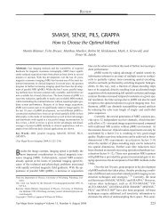
are plotted in Fig. 5. This simple plot conveys a
wealth of information. We have chosen to plot E
2 2 2 on a log scale versus g Ž 3 . , and thus
from Eq. 51 we see that each data set is a
straight line with a slope given by D, where D
is the respective diffusion coefficient of the species
in question. Of course, we could have just plotted
our data against the experimental variable, but by
2 2 2 using g Ž 3. as the abscissa, data acquired
using different experimental conditions are
more easily compared. It can be clearly seen that
as the diffusion coefficient decreases Ži.e.,
larger
molecule andor more viscous solution . , the slope
decreases which experimentally is reflected by
less attenuation.
In all of the discussion above, the gradient
pulses have been taken to be rectangular. This is
more out of technical and mathematical convenience
than necessity. It should be mentioned
that in the PEG experiment the gradient pulses
do not have to be rectangular, and in fact to
minimize the generation of eddy currents, it may
be preferable to have nonrectangular pulses. Using
Eq. 49 ,
the effects of arbitrarily shaped gradient
pulses can be considered Ž 78. and the computations
can be conveniently performed by
simple modification of the Maple worksheet given
in the Appendix. Another commonly used and
totally equivalent means of solving Eq. 41 is to
substitute Eq. 44 ,
but where S is a function of t,
into Eq. 41 directly and solving for S to obtain
t
2 2 H
0
lnŽEŽ t.. D F dt. 52
In evaluating Eq. 52 , the applied field gradient
must be replaced by the effective field gradient,
g , such that the sign of the gradient is changed
eff
Figure 5 A plot of the simulated echo attenuation for determining the diffusion coefficient
of water Ž . and protein Ž . . The simulations were performed using Eq. 51 with
1H 8 1 1 1 2.6571 10 rad T s , g 0.2 T m , 100 ms, and ranging from 0 to
10 ms. The diffusion coefficient of water and the protein were taken to be 2.33 109 and
1 10 10 m 2 s 1 , respectively. As the diffusion coefficient increases, the slope of the line
increases. If lnŽ E. is plotted on a linear scale versus the same abscissa the slope is given by
D Žsee Eq. 51 . .