weighted and two stage least squares estimation of ... - Boston College
weighted and two stage least squares estimation of ... - Boston College
weighted and two stage least squares estimation of ... - Boston College
You also want an ePaper? Increase the reach of your titles
YUMPU automatically turns print PDFs into web optimized ePapers that Google loves.
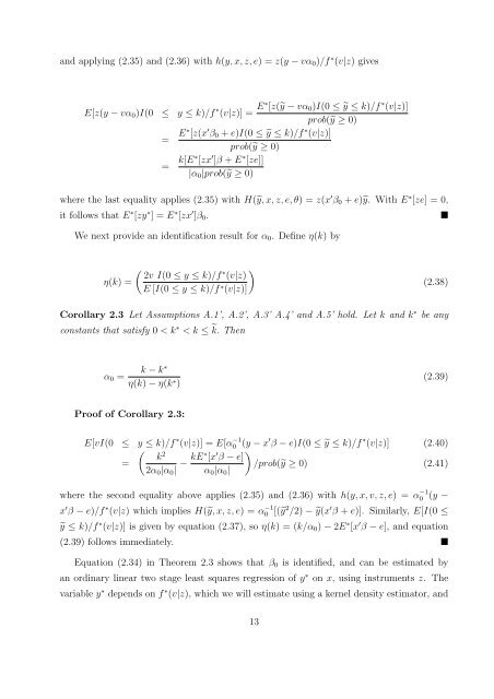
<strong>and</strong> applying (2.35) <strong>and</strong> (2.36) with h(y, x, z, e) = z(y − vα0)/f ∗ (v|z) gives<br />
E[z(y − vα0)I(0 ≤ y ≤ k)/f ∗ (v|z)] = E∗ [z(y − vα0)I(0 ≤ y ≤ k)/f ∗ (v|z)]<br />
prob(y ≥ 0)<br />
= E∗ [z(x ′ β0 + e)I(0 ≤ y ≤ k)/f ∗ (v|z)]<br />
prob(y ≥ 0)<br />
= k[E∗ [zx ′ ]β + E ∗ [ze]]<br />
|α0|prob(y ≥ 0)<br />
where the last equality applies (2.35) with H(y, x, z, e, θ) = z(x ′ β0 + e)y. With E ∗ [ze] = 0,<br />
it follows that E ∗ [zy ∗ ] = E ∗ [zx ′ ]β0. <br />
We next provide an identification result for α0. Define η(k) by<br />
η(k) =<br />
∗ 2v I(0 ≤ y ≤ k)/f (v|z)<br />
E [I(0 ≤ y ≤ k)/f ∗ <br />
(v|z)]<br />
(2.38)<br />
Corollary 2.3 Let Assumptions A.1’, A.2’, A.3’ A.4’ <strong>and</strong> A.5’ hold. Let k <strong>and</strong> k ∗ be any<br />
constants that satisfy 0 < k ∗ < k ≤ k. Then<br />
α0 =<br />
k − k ∗<br />
η(k) − η(k ∗ )<br />
Pro<strong>of</strong> <strong>of</strong> Corollary 2.3:<br />
(2.39)<br />
E[vI(0 ≤ y ≤ k)/f ∗ (v|z)] = E[α −1<br />
0 (y − x ′ β − e)I(0 ≤ y ≤ k)/f ∗ (v|z)] (2.40)<br />
2 k<br />
=<br />
2α0|α0| − kE∗ [x ′ <br />
β − e]<br />
/prob(y ≥ 0) (2.41)<br />
α0|α0|<br />
where the second equality above applies (2.35) <strong>and</strong> (2.36) with h(y, x, v, z, e) = α −1<br />
0 (y −<br />
x ′ β − e)/f ∗ (v|z) which implies H(y, x, z, e) = α −1<br />
0 [(y 2 /2) − y(x ′ β + e)]. Similarly, E[I(0 ≤<br />
y ≤ k)/f ∗ (v|z)] is given by equation (2.37), so η(k) = (k/α0) − 2E ∗ [x ′ β − e], <strong>and</strong> equation<br />
(2.39) follows immediately. <br />
Equation (2.34) in Theorem 2.3 shows that β0 is identified, <strong>and</strong> can be estimated by<br />
an ordinary linear <strong>two</strong> <strong>stage</strong> <strong>least</strong> <strong>squares</strong> regression <strong>of</strong> y ∗ on x, using instruments z. The<br />
variable y ∗ depends on f ∗ (v|z), which we will estimate using a kernel density estimator, <strong>and</strong><br />
13


