weighted and two stage least squares estimation of ... - Boston College
weighted and two stage least squares estimation of ... - Boston College
weighted and two stage least squares estimation of ... - Boston College
You also want an ePaper? Increase the reach of your titles
YUMPU automatically turns print PDFs into web optimized ePapers that Google loves.
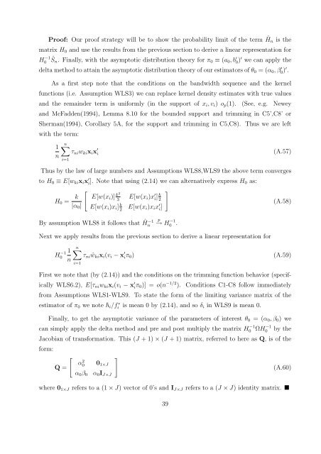
Pro<strong>of</strong>: Our pro<strong>of</strong> strategy will be to show the probability limit <strong>of</strong> the term ˆ Hn is the<br />
matrix H0 <strong>and</strong> use the results from the previous section to derive a linear representation for<br />
H −1<br />
0 ˆ Sn. Finally, with the asymptotic distribution theory for π0 ≡ (a0, b ′ 0) ′ we can apply the<br />
delta method to attain the asymptotic distribution theory <strong>of</strong> our estimators <strong>of</strong> θ0 = (α0, β ′ 0) ′ .<br />
As a first step note that the conditions on the b<strong>and</strong>width sequence <strong>and</strong> the kernel<br />
functions (i.e. Assumption WLS3) we can replace kernel density estimates with true values<br />
<strong>and</strong> the remainder term is uniformly (in the support <strong>of</strong> xi, vi) op(1). (See, e.g. Newey<br />
<strong>and</strong> McFadden(1994), Lemma 8.10 for the bounded support <strong>and</strong> trimming in C5’,C8’ or<br />
Sherman(1994), Corollary 5A, for the support <strong>and</strong> trimming in C5,C8). Thus we are left<br />
with the term:<br />
1<br />
n<br />
n<br />
i=1<br />
τniwkixix ′ i<br />
(A.57)<br />
Thus by the law <strong>of</strong> large numbers <strong>and</strong> Assumptions WLS8,WLS9 the above term converges<br />
to H0 ≡ E[wkixix ′ i]. Note that using (2.14) we can alternatively express H0 as:<br />
H0 = k<br />
<br />
E[w(xi)]<br />
|α0|<br />
k2<br />
3 E[w(xi)x ′ i] k<br />
2<br />
<br />
E[w(xi)xi] k<br />
2 E[w(xi)xix ′ i]<br />
By assumption WLS8 it follows that ˆ H −1<br />
n<br />
p<br />
→ H −1<br />
0 .<br />
Next we apply results from the previous section to derive a linear representation for<br />
H −1 1<br />
0<br />
n<br />
(A.58)<br />
n<br />
τni ˆwkixi(vi − x ′ iπ0) (A.59)<br />
i=1<br />
First we note that (by (2.14)) <strong>and</strong> the conditions on the trimming function behavior (specif-<br />
ically WLS6.2), E[τniwkixi(vi − x ′ iπ0)] = o(n −1/2 ). Conditions C1-C8 follow immediately<br />
from Assumptions WLS1-WLS9. To state the form <strong>of</strong> the limiting variance matrix <strong>of</strong> the<br />
estimator <strong>of</strong> π0 we note i/f ∗ i is mean 0 by (2.14), <strong>and</strong> so δi in WLS9 is mean 0.<br />
Finally, to get the asymptotic variance <strong>of</strong> the parameters <strong>of</strong> interest θ0 = (α0, β0) we<br />
can simply apply the delta method <strong>and</strong> pre <strong>and</strong> post multiply the matrix H −1<br />
0 ΩH −1<br />
0 by the<br />
Jacobian <strong>of</strong> transformation. This (J + 1) × (J + 1) matrix, referred to here as Q, is <strong>of</strong> the<br />
form:<br />
Q =<br />
α 2 0 01×J<br />
α0β0 α0IJ×J<br />
<br />
(A.60)<br />
where 01×J refers to a (1 × J) vector <strong>of</strong> 0’s <strong>and</strong> IJ×J refers to a (J × J) identity matrix. <br />
39


