weighted and two stage least squares estimation of ... - Boston College

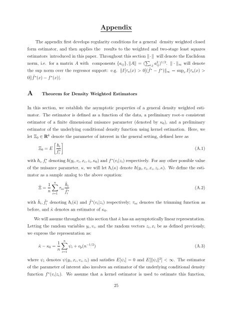
Appendix
The appendix first develops regularity conditions for a general density weighted closed
form estimator, and then applies the results to the weighted and two-stage least squares
estimators introduced in this paper. Throughout this section · will denote the Euclidean
norm, i.e. for a matrix A with components {aij}, A = (
i,j a2 ij) 1/2 . · ∞ will denote
the sup norm over the regressor support: e.g. I[τn(x) > 0]( ˆ f ∗ − f ∗ )∞ = sup x I[τn(x) >
0]| ˆ f ∗ (x) − f ∗ (x)|.
A Theorem for Density Weighted Estimators
In this section, we establish the asymptotic properties of a general density weighted esti-
mator. The estimator is defined as a function of the data, a preliminary root-n consistent
estimator of a finite dimensional nuisance parameter (denoted by κ0), and a preliminary
estimator of the underlying conditional density function using kernel estimation. Here, we
let Ξ0 ∈ Rk denote the parameter of interest in the general setting, defined here as
i
Ξ0 = E
f ∗ i
(A.1)
with i, f ∗ i denoting (yi, vi, xi, zi, κ0) and f ∗ (vi|zi) respectively. For any other possible value
of the nuisance parameter, κ, we will let i(κ) denote (yi, vi, xi, zi, κ). We define the esti-
mator as a sample analog to the above equation:
ˆΞ = 1
n
n
ˆi
τni
ˆf i=1
∗ i
(A.2)
with ˆ i, ˆ f ∗ i denoting i(ˆκ) and ˆ f ∗ (vi|zi) respectively; τni denotes the trimming function as
before, and ˆκ denotes an estimator of κ0.
We will assume throughout this section that ˆκ has an asymptotically linear representation.
Letting the random variables yi, vi, and the random vectors zi, xi be as defined previously,
we express the representation as:
ˆκ − κ0 = 1
n
n
i=1
ψi + op(n −1/2 ) (A.3)
where ψi denotes ψ(yi, xi, vi, zi) and satisfies E[ψi] = 0 and E[ψi 2 ] < ∞. The estimator
of the parameter of interest also involves an estimator of the underlying conditional density
function f ∗ (vi|zi). We assume that a kernel estimator is used to estimate this function,
25