weighted and two stage least squares estimation of ... - Boston College

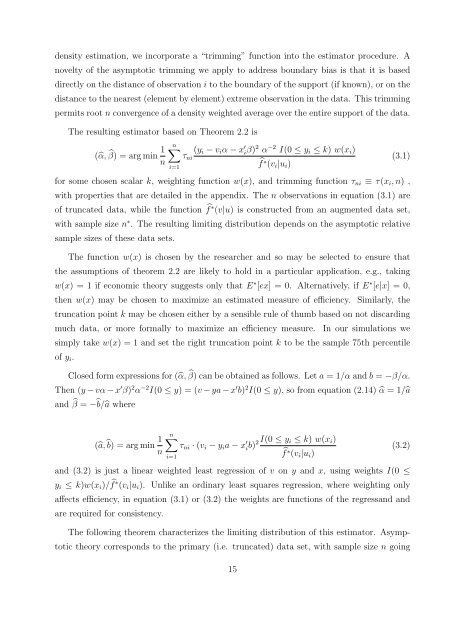
density estimation, we incorporate a “trimming” function into the estimator procedure. A
novelty of the asymptotic trimming we apply to address boundary bias is that it is based
directly on the distance of observation i to the boundary of the support (if known), or on the
distance to the nearest (element by element) extreme observation in the data. This trimming
permits root n convergence of a density weighted average over the entire support of the data.
The resulting estimator based on Theorem 2.2 is
(α, β) = arg min 1
n (yi − viα − x
τni
n
′ iβ) 2 α−2 I(0 ≤ yi ≤ k) w(xi)
f ∗ (vi|ui)
i=1
(3.1)
for some chosen scalar k, weighting function w(x), and trimming function τni ≡ τ(xi, n) ,
with properties that are detailed in the appendix. The n observations in equation (3.1) are
of truncated data, while the function f ∗ (v|u) is constructed from an augmented data set,
with sample size n ∗ . The resulting limiting distribution depends on the asymptotic relative
sample sizes of these data sets.
The function w(x) is chosen by the researcher and so may be selected to ensure that
the assumptions of theorem 2.2 are likely to hold in a particular application, e.g., taking
w(x) = 1 if economic theory suggests only that E ∗ [ex] = 0. Alternatively, if E ∗ [e|x] = 0,
then w(x) may be chosen to maximize an estimated measure of efficiency. Similarly, the
truncation point k may be chosen either by a sensible rule of thumb based on not discarding
much data, or more formally to maximize an efficiency measure. In our simulations we
simply take w(x) = 1 and set the right truncation point k to be the sample 75th percentile
of yi.
Closed form expressions for (α, β) can be obtained as follows. Let a = 1/α and b = −β/α.
Then (y − vα − x ′ β) 2 α −2 I(0 ≤ y) = (v − ya − x ′ b) 2 I(0 ≤ y), so from equation (2.14) α = 1/a
and β = − b/a where
(a, b) = arg min 1
n
n
i=1
τni · (vi − yia − x ′ ib) 2 I(0 ≤ yi ≤ k) w(xi)
f ∗ (vi|ui)
(3.2)
and (3.2) is just a linear weighted least regression of v on y and x, using weights I(0 ≤
yi ≤ k)w(xi)/ f ∗ (vi|ui). Unlike an ordinary least squares regression, where weighting only
affects efficiency, in equation (3.1) or (3.2) the weights are functions of the regressand and
are required for consistency.
The following theorem characterizes the limiting distribution of this estimator. Asymp-
totic theory corresponds to the primary (i.e. truncated) data set, with sample size n going
15