Module 5 - E-Courses
Module 5 - E-Courses
Module 5 - E-Courses

You also want an ePaper? Increase the reach of your titles
YUMPU automatically turns print PDFs into web optimized ePapers that Google loves.
Reliability Engineering Prof. G. L. Sivakumar Babu<br />
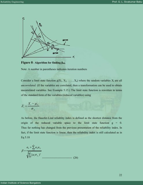
Figure<br />
8 - Algorithm for finding βHL<br />
Indian Institute of Science Bangalore<br />
Note: A number in parentheses indicates iteration numbers<br />
Consider a limit state function g(X1, X2, . . . , Xn) where the random variables Xi are all<br />
uncorrelated. (If the variables are correlated, then a transformation can be used to obtain<br />
uncorrelated variables. See Example 5.15.) The limit state function is rewritten in terms<br />
of the standard form of the variables (reduced variables) using<br />
Z<br />
i<br />
=<br />
X i<br />
− µ<br />
σ<br />
X i<br />
X i<br />
As before, the Hasofer-Lind reliablity index is defined as the shortest distance from the<br />
origin<br />
of the reduced variable space to the limit state function g = 0.<br />
Thus far nothing has changed from the previous presentation of the reliability index. In<br />
fact, if the limit state function is linear, then the reliability index is still calculated as in<br />
Eq 5.18<br />
a<br />
β =<br />
0<br />
+<br />
n<br />
∑<br />
i=<br />
1<br />
n<br />
∑<br />
i=<br />
1<br />
i<br />
a µ<br />
i<br />
X i<br />
X i<br />
( a σ )<br />
2<br />
-------------------------------- (26)<br />
22