Automatic Pouring Robot Project Progress Report for ECSE-4962 ...

Automatic Pouring Robot
Project Progress Report for ECSE-4962 Control
Systems Design
Akilah Harris-Williams
Adam Olmstead
Philip Pratt-Szeliga
Will Roantree
March 30, 2005
Rensselaer Polytechnic Institute

Abstract
This report contains our progress towards the develop of a prototype system to smoothly pour
water from a bottle into a cup using closed-loop control. Progress is being made towards the
completion of the system. After some delays, the mechanical system is nearing completion.
We are also nearing completion of the non-linear model. This includes compensation of the
variable intertia and center of mass of the bottle. Initial control has begun on a model
linearized about the point of highest inertia. Finally, the sensor subsystem can now acquire
and process images on the fly. We are looking to complete the system by the end of the
semester.

Contents
1 Introduction 4
2 Preliminary Results 5
2.1 Physical System Design and Construction . . . . . . . . . . . . . . . . . . . 5
2.2 System Modeling and Parameter Identification . . . . . . . . . . . . . . . . . 6
2.2.1 Inertia Identification . . . . . . . . . . . . . . . . . . . . . . . . . . . 6
2.2.2 Friction Identification . . . . . . . . . . . . . . . . . . . . . . . . . . . 7
2.2.3 Linearized Model . . . . . . . . . . . . . . . . . . . . . . . . . . . . . 10
2.3 Model Verification . . . . . . . . . . . . . . . . . . . . . . . . . . . . . . . . 11
2.4 Controller Design . . . . . . . . . . . . . . . . . . . . . . . . . . . . . . . . . 13
2.5 Sensor Development . . . . . . . . . . . . . . . . . . . . . . . . . . . . . . . 15
2.5.1 Image Acquisition . . . . . . . . . . . . . . . . . . . . . . . . . . . . . 15
2.5.2 Image Processing . . . . . . . . . . . . . . . . . . . . . . . . . . . . . 17
3 Summary of Progress 19
3.1 Plan . . . . . . . . . . . . . . . . . . . . . . . . . . . . . . . . . . . . . . . . 19
3.2 Schedule . . . . . . . . . . . . . . . . . . . . . . . . . . . . . . . . . . . . . . 19
3.3 Cost . . . . . . . . . . . . . . . . . . . . . . . . . . . . . . . . . . . . . . . . 21
3.4 Unanticipated Challenges . . . . . . . . . . . . . . . . . . . . . . . . . . . . . 22
3.5 Prognosis . . . . . . . . . . . . . . . . . . . . . . . . . . . . . . . . . . . . . 23
4 Statement of Contribution 24
A Mechanical System SolidWorks 26
B Simulation Block Diagrams 27
C Friction ID MATLAB Code 29
C.1 Static Friction Identification . . . . . . . . . . . . . . . . . . . . . . . . . . . 29
C.2 Coulomb and Viscous Friction Identification . . . . . . . . . . . . . . . . . . 31
D Image Acquisition MATLAB Code 34
E Image Processing MATLAB Code 36
1

List of Figures
2.1 Model Coordinate System . . . . . . . . . . . . . . . . . . . . . . . . . . . . 7
2.2 Simulink Diagram for Friction Identification . . . . . . . . . . . . . . . . . . 8
2.3 Friction Identification Data for Pan Axis . . . . . . . . . . . . . . . . . . . . 9
2.4 Orientation of Bottle for Linearization . . . . . . . . . . . . . . . . . . . . . 10
2.5 Simulation Results for 100 mL of Water . . . . . . . . . . . . . . . . . . . . 12
2.6 Simulation Results for 500 mL of Water . . . . . . . . . . . . . . . . . . . . 13
2.7 Step Response . . . . . . . . . . . . . . . . . . . . . . . . . . . . . . . . . . . 15
2.8 Frequency Response . . . . . . . . . . . . . . . . . . . . . . . . . . . . . . . 15
2.9 Color Detection with Threshold Values . . . . . . . . . . . . . . . . . . . . . 17
2.10 Color Detection with Modified Threshold Values . . . . . . . . . . . . . . . . 18
A.1 SolidWorks Model . . . . . . . . . . . . . . . . . . . . . . . . . . . . . . . . . 26
B.1 Simulink Diagram of Pan-Tilt Simulation: Complete System . . . . . . . . . 27
B.2 Simulink Diagram of Pan-Tilt Simulation: Pan-Tilt System . . . . . . . . . . 27
B.3 Simulink Diagram of Pan-Tilt Simulation: Pan-Tilt Dynamics Subsystem . . 28
B.4 Simulink Diagram of Pan-Tilt Simulation: Gravity Loading Subsystem . . . 28
2

List of Tables
2.1 Identified Friction Data . . . . . . . . . . . . . . . . . . . . . . . . . . . . . . 9
2.2 Webcam Timing Data . . . . . . . . . . . . . . . . . . . . . . . . . . . . . . 16
2.3 Image Processing Threshold Values . . . . . . . . . . . . . . . . . . . . . . . 18
3.1 Updated Schedule . . . . . . . . . . . . . . . . . . . . . . . . . . . . . . . . . 21
3.2 Parts . . . . . . . . . . . . . . . . . . . . . . . . . . . . . . . . . . . . . . . . 22
3.3 Raw Materials . . . . . . . . . . . . . . . . . . . . . . . . . . . . . . . . . . . 22
3.4 Labor Costs . . . . . . . . . . . . . . . . . . . . . . . . . . . . . . . . . . . . 22
3

Chapter 1
Introduction
The Automatic Pouring Robot will smoothly pour a user-specified amount of water from a
bottle into a cup using closed-loop control. We are aiming to design a system that can pour
the desired amount of liquid within 10 mL of the desired value. We also want to pour at a
reasonable rate, such that the cup could be filled in 20 seconds, corresponding to a flow rate
of 45 mL/s. Some industrial applications addressed by this problem include pouring molten
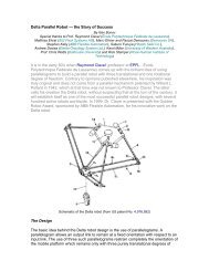
metal into casting and pouring hazardous materials or chemicals. A currently available
commercial product for a similar task is the D&A101 Autopour, which pours molten metal
into piston gravity castings.[5] The Autopour uses an open-loop controller to tilt the ladle.
To accomplish our task, we will mount a bottle on a pan/tilt mechanism with MATLAB /
Simulink controlled motors. Models of the bottle, the tilt mechanism and the water inside
the bottle will be created in SolidWorks. Using Visual Basic and the SolidWorks API, we
will calculate mass and inertial tensor properties of each model for varying tilt angles and
water volumes. [2] From these properties we will interpolate a dynamic model of the system
and then design a closed-loop controller.
During the pour, volume updates to the dynamic model are required. To do this update we
will measure the cup water volume and subtract this measurement from the initial bottle
water volume. Measurement of the cup water volume will be accomplished using a webcam.
Using a color detection algorithm, the webcam will measure the current height of the cup
water and MATLAB will calculate the cup water volume.
This problem is a challenging one due to a variety of factors. The system’s gravity loading
changes constantly with time, due to the liquid’s motion within the bottle. Also, by making
the pouring system closed loop, as opposed to the strictly open loop solutions currently
available, we are stepping into new grounds. There is also a fair amount of sensor error, so
designing a finely tuned controller to pour the desired amount of liquid will be a challenging
task.
4

Chapter 2
Preliminary Results
2.1 Physical System Design and Construction
The mechanical system, as previously discussed, went through a series of evolutions. The
final design was chosen because it kept the system as compact as possible, reducing rotating
mass and material needed to construct it. The pieces that are attached to the frame, the
gears, motors, and bottle, were all placed within a somewhat tight tolerance of each other
in order to accomplish this. Although these pieces can come in very close contact with each
other, they never actually meet, and thus, the system is as compact as it can be.
The first step in constructing the mechanical system was getting the side pieces for the tilt,
the base for the tilt, and the base for the pan machined. These pieces can be seen as the
aluminum pieces in the figure of the entire mechanical system shown in Appendix A. Many
options were examined when considering the machining of these pieces, and the decided upon
approach was to use the school’s waterjet. The waterjet can cut metal with great precision,
based on the CAD drawings. Since the mechanism was full of sometimes complex geometry
that had to be machined perfectly, we decided the waterjet was the best approach, not only
because of its precision, but also because of the speed with which it operates. An unforeseen
challenge that presented itself with this approach, however, was user error. Having used the
waterjet with a different operator previous to CSD, we were familiar with its use. However,
for this project, we had to contact use a different person. Although the actual cutting with
the waterjet took less than an hour, the process itself took almost 3 weeks. The operator
was given the CAD drawings, and it took a week for him to get to them. When he cut
them the first time, he cut them the wrong size. As he did not cut them until spring break,
we did not find out until a week later. Once this problem was discovered, he was given the
CAD drawings again, and another week later, we had the final pieces. The total price for
machining with the waterjet was $35, a good bit less than the original estimate of $50-100.
The pieces were taken to the lab once they were acquired. Rafael assisted us in drilling the
proper holes for construction. Holes were drilled for the attachment of bearings, encoders,
5

and axles. Some of the tolerances on the waterjet were off, and so some of the pieces had
to be drilled or milled where a waterjet had already cut a hole or slot. This, again, was an
unforeseen challenge, but easily overcome.
2.2 System Modeling and Parameter Identification
The modeling of our system is particularly unique. Rather than modeling an object with a
constant properties, our system has variable inertia. This is due to the fact that the water
moves around in the bottle as the tilt angle is increased. In addition to this, as liquid is
poured out of the bottle, the volume of water, and therefore overall mass, changes. This
results in a system with both variable values of inertia and center of mass.
To deal with this problem, an automated program was written to find the changing mass
properties of the bottle, the tilt mechanism and the water using the Solidworks API. The
mass properties found are the mass, center of mass, and principle moment of inertia. A nonlinear
Simulink model uses center of mass, mass and principle moment of inertia to simulate
gravity loading and frictional effects. To complete the simulation, the Coulomb and Viscous
friction for the final assembled mechanical system must be determined when its assembly is
finished.
2.2.1 Inertia Identification
A Visual Basic program to automate the extraction of center of mass, mass and moment
of inertia properties from Solidworks is operational. The program steps through the angles
1 ◦ , 10 ◦ , 20 ◦ , 30 ◦ , 40 ◦ , 50 ◦ , 60 ◦ , 70 ◦ , 80 ◦ , 89 ◦ , 91 ◦ , 100 ◦ , 110 ◦ , 120 ◦ , 130 ◦ , 140 ◦ , 150 ◦ , 160 ◦ ,
170 ◦ and 179 ◦ . For each of these angles, the program finds the height of water that will
match a volume of 100 mL, 200 mL, 300 mL, 400 mL and 500 mL. For each of these one
hundred data points, the program generates a lookup table matrix corresponding to center
of mass in the Z direction, mass and principle axis of inertia in the X direction. Figure 2.1
shows the coordinate system used in the modeling and simulation. The center of mass, mass
and principle axis of inertia for varying angles and volumes are determined, and this data
is entered into a 2D lookup table in Simulink, which interpolates the output value for any
intermediary input values that it may receive.
A non-linear Simulink model of the bottle, tilt mechanism and water is nearly complete.
The gravity loading subsystem is complete. It incorporates a changing mass and center of
mass in the Z direction. These properties change with respect to the current tilt angle and
the current volume of water in the bottle.
6

coordinate_system.bmp (BMP Image, 536x613 pixels) file://///sambasrv/prattp/public_html/controlsysdesign/papers/progr...
2.2.2 Friction Identification
Figure 2.1: Model Coordinate System
In order to get an accurate non-linear model of the system, the friction in the system needs
to be identified. Friction exists between all moving parts in the system, such as the axle and
the bearings, the belts and the pulleys, and even inside the motors. If accurately determined,
this friction can be accounted for and cancelled in the model. There are three types of friction
in the system that we will estimate experimentally: static, coulomb and viscous.
Static friction, sometimes referred to as “stiction,” is the force that exists between any two
objects at rest. This friction must be overcome before the object(s) can move. In our case,
static friction exists between the bearings and the axle. To experimentally determine this
value, xPC target was used to interface with the motors, using the Simulink diagram shown
below in Figure 2.2. A script was then used, which simply applies various constant torque
1 of 1 3/30/2005 2:35 PM
values, until the axle begins to rotate. First, a coarse pass was done in torque increments
of 0.01 Nm. Then, once the axle rotates, a finer pass was done in 0.001 Nm increments to
find the value of the static friction to the nearest 0.001 Nm. The script used to identify the
7

static friction is shown in Appendix C.1.
Step
Step1
Step2
Step3
−K−
Gain1
−K−
Gain3
Saturation
Saturation1
1PCIM−DAS1602/16
ComputerBoards
2 Analog Output
PCI−QUAD04
Comp. Boards
Inc. Encoder
PCI−QUAD04
PCIM−DAS1602 16 PCI−QUAD04
Comp. Boards
Inc. Encoder
PCI−QUAD04 1
Count
Count
2*pi/(1024*4)
2*pi/(1024*4)
Gain2
Figure 2.2: Simulink Diagram for Friction Identification
Gain
3
Pos1
4
Out1
K (z−1)
Ts z
Discrete Derivative
K (z−1)
Ts z
Discrete Derivative1
Once the static friction is determined, a different script is used to determine the coulomb
and viscous friction values for the pan axis. Using the same Simulink diagram, this script
measures the velocity with respect to time for a range of input torques. An initial, hightorque
(10 V for 0.25s) pulse is given to the motor to break static friction, and then the
desired torque was applied. Then the velocity values are recorded for 10 seconds, as the
motor to settles to its steady-state velocity.
For each constant input torque, the recorded velocity values are passed through a lowpass
filter to remove noise, and then a steady-state value is determined by averaging the last 10%
of the values together. The coulomb friction is the first torque value at which the steadystate
velocity is non-zero, within a specified tolerance. The viscous friction is the slope of
the least-squares best fit line of torque vs. steady-state velocity for all nonzero values of the
latter. [6] The MATLAB code used to generate the friction data is shown in Appendix C.2.
The results for the initial friction testing on the unloaded pan axis are summarized below in
Table 2.1. This table shows the identified friction values for the pan axis. Only this axis has
been tested because the mechanical system has not been completed, and we cannot therefore
test it for the final friction values. The torque versus steady-state velocity plot used to find
these values is shown below in Figure 2.3.
8
Vel1
1
2
Vel2

Applied Torque (Nm)
0.15
0.1
0.05
0
−0.05
−0.1
−0.15
Static
Forward Reverse
Pan 0.078 Nm 0.076 Nm
Tilt N/A N/A
Coulomb
Forward Reverse
Pan 0.05573 Nm 0.06251 Nm
Tilt N/A N/A
Viscous
Pan
Forward
8.0146x10
Reverse
−4 Nm s
rad
9.1426x10−4 Nm s
Tilt N/A
rad
N/A
Table 2.1: Identified Friction Data
Torque vs. Steady−State Velocity
−0.2
−50 −40 −30 −20 −10 0 10 20 30 40 50
Steady−State Velocity (rad/s)
Figure 2.3: Friction Identification Data for Pan Axis
9

2.2.3 Linearized Model
The above Simulink models represents the full, non-linear model of our system. However,
when designing the controller, we must linearize the model to simplify the design process.
The dynamics of our system are particularly hard to model due to the changing inertia.
Therefore, we will design for the worst case in our controller, so the system is linearized
about the point with the highest inertia. The equation of motion for the model is:
(Ixx + N 2 Im) ¨ Θ = mg cos( π
2 + α − Θ) − (Fv ˙ Θ + Fcsgn( ˙ Θ)) (2.1)
The strategy we used to create the linear model is to linearize the non-linear model about
a tilt angle and water volume when the inertia is largest. The angle and water volume we
have linearized about is 90◦ linear_bottle.bmp (BMP Image, 583x350 and pixels) 500 mL respectively. file://///sambasrv/prattp/public_html/controlsysdesign/papers/progr...
This orientation is shown in Figure
2.4
Figure 2.4: Orientation of Bottle for Linearization
This results in the system described by the state-space model shown in Equation 2.2.
˙x =
⎡
0
⎢
⎣ 0
0
0
⎤ ⎡ ⎤
0
1
⎥ ⎢ ⎥
−0.0001 ⎦ x + ⎣ 0 ⎦ u
0 0.001
y =
−4.454 1
0 0 1
x
10
(2.2)

2.3 Model Verification
To verify the non-linear model of our system, simulations were run using Simulink. The
block diagrams of the system contained in Appendix B show the Simulink block diagrams
that represent our system. An initial simulation of tilt angle for the new mechanical system
incorporating tentative friction values and gravity is complete. In simulation, the bottle
can rotate from 0 to 180 degrees and a volume of 0 to 500 milliliters of water can be
selected. Compared to the draft simulation in the project proposal, the current simulation
has improved. The equations of motion for gravity loading are now understood. The parallel
axis theorem is applied to the moment of inertia to align it with the output coordinate system.
Two initial simulations of the tilt angle, Θ, including changing center of mass, mass and
moment of inertia have been completed. These simulations were run and verified intuitively
to make sure that the results make sense. The two simulations are for a bottle holding water
volumes of 100 mL and 500 mL respectively. Simulation plots for angular position (Θ),
angular velocity (ω), and angular acceleration (α) are shown in the figures below.
In the 100 mL simulation, the bottle begins at 0 ◦ and falls to a steady state of 48.1 ◦ past
vertical. Intuitively, this simulation result shown in Figure 2.5 is logical. At time zero,
gravity overcomes Coulomb friction and accelerates the motion of the bottle away from the
original position. Viscous friction slows the angular motion when velocity is nonzero and
acts with the dynamic gravity loading to settle theta. There is little inertia when filled with
100mL of water and oscillation past the steady state is minimal.
11

Angular Position (deg)
Angular Velocity (deg/s)
Angular Acceleration (deg/s²)
60
40
20
0
0 10 20 30
Time (s)
40 50 60
10
5
0
−5
0 10 20 30
Time (s)
40 50 60
10
5
0
−5
0 10 20 30
Time (s)
40 50 60
Figure 2.5: Simulation Results for 100 mL of Water
12

In the 500 mL simulation, the bottle begins at 0 ◦ , falls to 89 ◦ below the tilt axis, oscillates,
and rises back to a steady state of 53.4 ◦ . This simulation result is also logical. At time
zero, gravity overcomes Coulomb friction and accelerates the motion of the bottle away from
the original position. Before the max angular displacement, the large inertia effect pushes
the bottle past the horizontal. Viscous friction and the large gravity loading act to settle
theta. Shown below in Figure 2.6 is a plot of the angular displacement, angular velocity and
angular acceleration of the tilt axis for the 500mL simulation.
Angular Position (Deg)
Angular Velocity (Deg/s)
Angular Acceleration (Deg/s²)
100
50
0
0 10 20 30
Time (s)
40 50 60
40
20
0
−20
0 10 20 30
Time (s)
40 50 60
20
10
0
−10
0 10 20 30
Time (s)
40 50 60
2.4 Controller Design
Figure 2.6: Simulation Results for 500 mL of Water
Using the linear model discussed in section 2.2.3, a controller can be designed to control the
motion of the pan and tilt axes. The plant, is a complex model with dynamic gravity loading
based on changing inertia tensors. In a control sense, this means that the system’s poles will
be changing continually. Therefore, a robust controller is very desirable in this application.
The controller will be designed using frequency response methods, in conjunction with rootlocus
to determine the desired gain. This will allow us to design fairly large stability margins,
which are needed so that the moving poles don’t disrupt the control too greatly. [1] A
traditional PID controller does not allow this flexibility in designing the margins, as only
13

the gains are being tuned. In a lead/lag controller, the poles and zeros of the controller can
be moved around in addition to the gains, allowing the magnitude and phases of the plant
to be manipulated.
When designing the controller, it is important to keep in mind the controller specifications.
They include a small overshoot: less than 5%, a small settling time: less than 3% and a
steady-state error less than 0.1. Rise time is not a crucial factor for our design, because the
sensing subsystem responds much slower than the rest of the system, which necessitates a
relatively slow, smooth pouring. The controller is designed based on the worst case inertia
(largest) because of the constant movement, change in the center of mass, and change in the
water volume.
For the lead-lag compensator, we have to go through various equations to design the controller
to the specifications. The transfer function of a lead controller can be generalized as
follows:
W (s) =
1 + a1τ1s 1 + a2τ2s
1 + τ1s 1 + τ2s
where a1 < 1
a2 > 1
(2.3)
In order to get the phase angle, frequency and gain, the following equations below were used:
Phase Angle: Φmax = sin −1 ( a2 − 1
) − 5◦
a2 + 1
Frequency: ωm = 1
√
τ2 a2
(2.4)
(2.5)
Gain: (am)dB = (a1)dB + 1/2(a2)dB = (a1)dB + 1/2(1/a1)dB = 1/2(a1)dB (2.6)
The design process is then simply as follows:
1. Choose K to satisfy the steady-state requirements, K = 1
ess
2. Draw a Bode Diagram of KG(s)
3. Determine the new crossover frequency, ωc
Using this above design method, the following controller was designed. However, the system
that we are working with is a completely digital system. Therefore, our controller must be
discretized. The Bilinear (Tustin) transformation is used to discretize the above continuous
controller at a sampling frequency of 1 kHz using the Control System Toolbox. This emulation
design results in a discrete controller. The step response of this controller is shown
in Figure 2.7. As can be seen, the system responds slowly, but smoothly. This is consistent
with our requirements. The frequency response is shown in Figure 2.8.
14

step.bmp (BMP Image, 613x356 pixels) file:///C:/Documents%20and%20Settings/olmsta/Desktop/Dropbox/...
freq.bmp (BMP Image, 603x351 pixels) file:///C:/Documents%20and%20Settings/olmsta/Desktop/Dropbox/...
2.5 Sensor Development
2.5.1 Image Acquisition
Figure 2.7: Step Response
Figure 2.8: Frequency Response
Several systems that have tackled the pouring problem have all done so with an open loop
controller. However, we are providing feedback to the system with a webcam to determine
15
1 of 1 3/30/2005 6:08 PM

the volume currently in the cup. From this volume, the system will be able to determine
the desired angular position of the tilt axis. The correlation between the current volume
and the angular position will be done with an experimentally determined lookup table. Our
controller will track this position, and the bottle will pour in the process.
The first step of the sensor development is to acquire images from the webcam. To do so,
we are using MATLAB’s Image Acquisition Toolbox. A MATLAB script is used to grab
images from the webcam. A video input object is created, and it is configured to continually
take images as fast as possible with logging enabled. [3] As soon as an image is ready, it is
grabbed from memory and sent to the image processing function, which returns the highest
row of pixels filled with water. This data is sent to xPC target, where a lookup table is
used to correlate the pixel data to the actual volume, via the TCP/IP link. This process is
repeated continually. The script used to do this is shown in Appendix D.
The speed at which images can be grabbed and processed and sent to xPC target is the
bottleneck for the system. Therefore, the timing of the sensing is very important. Timing
tests were done to see how well the webcam performs in comparison to its nominal framerate
of 30 fps. First, the framerate was measured with no other operations performed. Then, the
camera was continually polled in MATLAB. Next, image processing was added to the test.
Finally, a test was done with acquisition, processing, and sending to xPC target. For each
case, the experiment was repeated 10 times, with each run acquiring 100 frames. The average
period and its standard deviation were determined. The timing results are summarized in
Table 2.2.
Mean Period Standard Deviation Average FPS
No Logging 68.3 ms 18.8 ms 14.63
Logging 70.9 ms 27.4 ms 14.1
Processing 71.0 ms 25.4 ms 14.09
xPC Communication 134.9 ms 75.2 ms 7.42
Table 2.2: Webcam Timing Data
As seen, the camera, even when only acquiring images and saving them to memory, runs at
14.64 fps, less than half of its advertised framerate. When the data is continually saved to
the workspace, the average period does not increase much, but the standard deviation of the
times increases drastically. Image processing, surprisingly has very little effect. However,
communication with xPC target proved to be a large bottleneck and inconsistency by both
halving the framerate and doubling the deviation. This is most likely due to the laptop
computer multitasking between TCP/IP communication and image acquisition in MATLAB.
To try and reduce this fluctuation, the image acquisition will be written as a function rather
than a script, so that it will be pre-compiled. Also, a T40 laptop will be used rather than
the T22 that was used for the timing testing.
The primary implication of this slow framerate is that the pouring speed will have to be
limited. If the system pours too quickly with a slow framerate, then there is a chance that
the system will over pour before the sensing subsystem can tell it that it went too far.
16

2.5.2 Image Processing
Once the images are acquired, they are sent to a function that determines the highest pixel
row. This data is later correlated to the volume. Color detection is used to determine this
value. This method finds the pixels that are red, as determined by a tunable threshold value
for component intensities. The images taken from the webcam are conveniently stored in
the RGB format, so we can look for pixels that have a high R component and lower G and
B components. [4] To facilitate this, the water used in this project will be dyed red with
food coloring, allowing the algorithm to search for red in the image. A downside to color
detection is a relatively high sensitivity to noise. For this reason, the viewing conditions are
fixed and the algorithm tuned to it. The cup will be completely surrounded by white to
improve contrast for the webcam.
The function to find the highest row of pixels is rather straightforward. The MATLAB code
can be found in Appendix E. First of all, since the webcam has a better horizontal resolution
than vertical resolution (288x352), the images will be rotated 90 ◦ clockwise from the upright
position. A certain band in the middle of the cup is focused on so that no pixels outside
the boundary of the cup will be considered. These boundaries have yet to be finalized, as
the fixed location of the webcam is yet to be decided. Then the average pixel value for each
column within these boundaries is found, and that value is applied to threshold component
color values. These values were determined on a sample setup. Figure 2.9 shows an the
image used to calibrate the threshold values. The image on the bottom is one where all
black pixels are those that were found to be “red” by the threshold values, with the original
shown on the top as a reference.
Original Image
(a) Original Image
Threshold Values Applied
(b) First Threshold Values Applied
Figure 2.9: Color Detection with Threshold Values
Figures 2.9 & 2.10 show the effect of different threshold values on the detection of the red
pixels. Just using a simple single set of threshold values results in the image in the first
figure. Notice how an area of the liquid is not detected, which is due to the way the light
17

Original Image
(a) Original Image
Second Threshold Values Applied
(b) Second Threshold Values Applied
Figure 2.10: Color Detection with Modified Threshold Values
shined on the cup when the image was taken. The second set of threshold values includes
an “or” for when the red value saturates. This helped improve detection of all the water
pixels, while not adding any new unwanted pixels. Table 2.3 below briefly summarizes the
threshold values use to detect the red pixels in the images above. These threshold values are
applied to the mean pixel of each row in the above
GT or LT Pixel Value or GT or LT Pixel Value
Red > 140 == 255
Green < 150 < 200
Blue < 140 < 160
Table 2.3: Image Processing Threshold Values
18

Chapter 3
Summary of Progress
3.1 Plan
The overall goal of our project has remained the same: to pour a specified amount of water
into a cup. Originally, we had hoped to pour the liquid very quickly into the cup. However,
we are limited by the speed of our sensing subsystem, which is only running at approximately
7.5 frames per second. Therefore, in order to maintain the accuracy of the pouring, we need
to slow it down.
In the proposal we also had plans to possibly move the cup’s location while not pouring and
have the system pan to the cup’s new position. However, our primary efforts are currently
on the accurate pouring with the tilt axis, and we will most likely not have the time to
implement this feature.
3.2 Schedule
Progress, with respect to the original schedule, has been uneven. A large portion of this is
due to the fact that the waterjet took much longer than expected (more than two weeks)
to get us the parts for the mechanical system. We only received the parts a few days prior
to the writing of this memo, but we are almost done with the assembly of the system. The
only remaining thing that we are waiting on for the completion of the mechanical system is
a tilt gear belt, which has been ordered. The only two tasks that still need to be done with
the mechanical system are to integrate the mechanical system with the pan-tilt mechanism,
and to mount the webcam to a fixed location so we can have accurate sensor data.
The delay in the mechanical system has caused delays in other areas as well. Most notably
is with the model validation. The final friction values have yet to be indentified, since the
19

system is not completed. We were unable to run any verification experiments with the model,
other than comparing the model to what “should” happen intuitively. This is a top priority
for the when the mechanical system is finished. The verification experiments that we run
will consist primarily of comparing actual data to the simulated data. Using xPC target,
we can collect position data from the encoders for the actual system when excited by an
arbitrary input. We will compare this data to the simulated position data, and iteratively
improve the model if needed. The various simulations that we will compare are the model
unloaded, with an initial amount of water in it, and the settling after excitation by a short
burst of constant torque.
The sensor development also has been delayed due to the incomplete mechanical system.
The MATLAB scripts have been developed and timing tests done for image acquisition and
processing. However, we were unable to correlate any of the pixel data to the volume.
The reason for this is that the webcam has yet to be mounted relative to the cup. It is
important for the webcam to be in a fixed location when this determination is done, to
ensure the accuracy of the sensing results. Due to the resolution of the camera, each pixel
row represents around 1.33 mL. Therefore, we need to keep it in a fixed location relative
to the cup to ensure that the data is consistent. This correlation will be determined by
pouring small increments of water into the cup (start with 5 mL increments, and make finer
if needed), and then running the image processing algorithm on it. Data will be collected
several times for each water level to average out any noise in the acquisition, and the data
will then be fit to a curve, or a lookup table in Simulink, depending on the characteristics
of the data. Once the webcam is mounted, we can also determine the boundaries that will
be used to ignore all image information outside the cup.
The model and control integration will begin shortly after the model is validated. Simulated
and actual results will be compared for the open and closed-loop response to various reference
inputs. We need to still complete the following cycle: test controller on integrated system,
iterate control design, and retest controller. Also, we need to generate a smooth trajectory
for the controller to follow to avoid high-frequency vibrations in our system. We will most
likely use a trapezoidal trajectory for our system to move from one point to an another.
The updated schedule is shown below in Table 3.1. This shows all of the tasks that still need
to be completed, and their new timeframes.
20

Table 3.1: Updated Schedule
Task Start Completion Leader
Develop Mechanical System
Fabricate new mechanical system 3/29/05 3/30/05 Will
Integrate new mechanical system with Pan-Tilt 3/31/05 3/31/05 Will
Friction Testing
Execute script with new mechanical design 4/1/05 4/4/05 Akilah
Incorporate friction data into existing model 4/4/05 4/5/05 Will
Image Processing
Correlate pixel data to beaker volume 3/30/05 3/31/05 Adam
Develop pixel data to volume model 4/1/05 4/4/05 Adam
Verify pixel data to volume model 4/4/05 4/5/05 Akilah
Incorporate data into existing model 4/6/05 4/7/05 Akilah
Simulation
Add volume feedback to Simulink 3/30/05 4/4/05 Phil
Experiment to get flow rates at various angles 4/1/05 4/4/05 Will
Test model in Simulink 4/7/05 4/11/05 Adam
Verify model on integrated system 4/11/05 4/13/05 Akilah
Controller Design
Tune lead-lag controller 4/13/05 4/15/05 All
Test controller in Simulink 4/15/05 4/21/05 All
Test controller on actual system 4/21/05 4/22/05 All
Iterate control design 4/25/05 4/26/05 All
Reports
Final report work 4/21/05 5/4/05 All
Final presentation work 4/21/05 5/4/05 All
3.3 Cost
The original cost schedule that was submitted for the proposal has proven to be accurate
thus far. Only two additions have been made, which are the waterjet machining, which cost
an additional $35, and a new tilt gear belt (which we were expecting to have provided, but
we needed a new size). We also need to increase the amount of time for each group member
on the project, as the original 50 will be insufficient for completing the project. An estimate
of 80 will replace it. The updated cost schedules for parts, raw materials, and labor are
shown below in Tables 3.2, 3.3 and 3.4, respectively.
21

Table 3.2: Parts
Item Quantity Cost Total Cost
Cup 1 $1.25 $1.25
Bottle 1 $1.45 $1.45
Red Dye 1 $1.00 $1.00
Logitech WebCam 1 $29.95 $29.95
3” Universal Exhaust Clamp 1 $3.24 $3.24
Pan Belt 1 $3.92 $3.92
Pan Gear A 1 $9.97 $9.97
Pan Gear B 1 $22.02 $22.02
Tilt Belt 1 $4.00 $4.00
Tilt Gear A 1 $7.95 $7.95
Tilt Gear B 1 $22.02 $22.02
Pittman Motor GM9234S017 2 $97.59 $195.18
Total $301.95
Table 3.3: Raw Materials
Item Quantity Cost Total Cost
1/4” Aluminum Plate 500 in 2 $0.16 /in 2 $80.00
Sand for Waterjet 1 $5.00 $5.00
Total $85.00
3.4 Unanticipated Challenges
Certain unanticipated challenges have presented themselves throughout the progress of this
report. The first, and most complex, is the modeling for the system. The inertia modeling
for this system has proven to be quite difficult. The differing inertia of the liquid in the
bottle has complicated the modeling to an unexpected degree. Although the difficulty of the
modeling of this system took us by surprise, we are certain that we have a grasp on it now.
The next unanticipated challenge was a problem with help from outside the course. In order
to maximize the accuracy of the machining of the mechanical system, it was decided that
the main parts of system would be machined using a waterjet, which is computer controlled,
Table 3.4: Labor Costs
Description Hours Cost Total Cost
Akilah Harris-Williams (Engineer) 80 $25.00 $2000
Adam Olmstead (Engineer) 80 $25.00 $2000
Philip Pratt-Szeliga (Engineer) 80 $25.00 $2000
Will Roantree (Engineer) 80 $25.00 $2000
Jim Schatz (Waterjet Operator) 1 $30.00 $30.00
Total $8030
22

and driven by engineering drawings. The parts were ready to be returned a week after
the material and the drawings were dropped off with the operator, even though the actual
machining took less than an hour. Unfortunately, the parts were ready to be returned at
the beginning of spring break, when no one was around to receive them. When the group
members returned from the break, and got the parts, it was discovered that they were
machined incorrectly, and needed to be machined again. This took another week, turning
an hours worth of work into a 3 week process.
Another unanticipated challenge was with the machining of the mechanical system. When
the waterjet cuts pieces of aluminum plate, it does not leave a perpendicular edge. Instead,
it leaves a slight angle. For most applications, this is inconsequential. However, for this
system, the bottom edges of the sides of the tilt mechanism were stricken with this angle,
and had to be further machined, as they are supposed to sit flat against the base of the tilt
mechanism. When the TA was assisting us with this process, there was a problem with the
mill, delaying progress of the system for a few hours. Once the problem was resolved, the
parts were machined correctly, and the system was assembled.
Finally, the control design is also more challenging than expected. This is due exclusively to
the complexity and dynamic nature of our system. The variable inertia has made it difficult
to design a controller that is robust enough to pour quickly in one case without overshooting
too much in another case. For this reason, we may have to pour fairly slowly in cases where
it is not needed.
3.5 Prognosis
Our forecast for the remainder of the project is that the system will be able to pour liquid
into a cup, as originally specified in the design memo. The system will not have any of the
proposed additions, due to a limited time budget. However, provided that certain obstacles
are overcome, the group feels confident in its ability to complete a system that will accurately
pour liquid into a cup, without spilling, while tracking the amount that is being poured.
23

Chapter 4
Statement of Contribution
Akilah worked on the controller design and tuning. This includes linearizing the model about
the operation point and designing the lead-lag controller.
Adam worked on the friction identification, the webcam development including acquisition
and processing. He also worked on the organization, formatting, and proofreading of this
report, and the Plan, the Cost, test procedures in Schedule, and part of the Unanticipated
Challenges sections.
Phil worked on the modeling and. This includes developing the Simulink block diagram
for the non-linear model, identification of the inertia and center of mass properties from
SolidWorks, and gravity and friction simulation of the model. He also updated the schedule.
Will worked on the design of the mechanical system, getting the parts machined, assembling
the system, and did some threshold value tuning on the webcam. Also wrote the majority
of Unanticipated Challenges and Prognosis.
Akilah Harris-Williams Adam Olmstead
Phil Pratt-Szeliga Will Roantree
24

Bibliography
[1] Prof. Joe Chow. Course notes. Control System Engineering, 2004.
[2] SolidWorks Corporation. Api support. http://www.solidworks.com/pages/services/
APISupport.html.
[3] The MathWorks Inc. Image acquisition toolbox user’s guide. http://www.mathworks.
com/access/helpdesk/help/toolbox/imaq/.
[4] The MathWorks Inc. Image processing toolbox user’s guide. http://www.mathworks.
com/access/helpdesk/help/toolbox/images/.
[5] Dana Advanced Automated Systems. Casting robot d&a101. http://www.novindana.
com/da101.shtml.
[6] Prof. John Wen. Lecture 4. Control System Design Course Notes, 2005.
25

Appendix A
Mechanical System SolidWorks
Figure A.1: SolidWorks Model
26

Appendix B
Simulation Block Diagrams
Set Parameters
0
Input Torque
0.0001
Original Volume
1
tau
2
volume
Saturation
tau
volume
theta
volume_out
Pan−tilt dynamics
theta
volume
Image Processing Simulation
volume_out
Figure B.1: Simulink Diagram of Pan-Tilt Simulation: Complete System
tau
theta
thetadot
volume
Subsystem
thetaddot
volume_out
180/pi
Gain
theta_ddot
To Workspace2
Theta2 ddot scope
1
s
thetaddot −> thetadot
1
s
thetadot−>theta
theta_dot
To Workspace
Theta2 dot scope
Saturation
(180 deg)
Figure B.2: Simulink Diagram of Pan-Tilt Simulation: Pan-Tilt System
27
180/pi
Gain1
180/pi
Gain2
1
theta
2
volume_out
Terminator
theta
To Workspace1
Theta2 scope

2
theta
3
thetadot
4
volume
1
tau
theta
volume
G(theta)
Gravity Load
thetadot Friction Matix
F(qdot)
IXX
u[1]/(u[2]+N2^2*Im2)
2
volume_out
Fcn1
1
thetaddot
Figure B.3: Simulink Diagram of Pan-Tilt Simulation: Pan-Tilt Dynamics Subsystem
2
1
theta
volume
center of mass Z (u[1])
mB (u[2])
−u[2]*g*u[1]
Figure B.4: Simulink Diagram of Pan-Tilt Simulation: Gravity Loading Subsystem
28
G2
1
G(theta)

Appendix C
Friction ID MATLAB Code
C.1 Static Friction Identification
% Adam Olmstead
% Team 1 ECSE-4692
% Static Friction Identification
% 2-28-05
% Initialize Variables
torque_sat=1.0557;
stat_fric=zeros(1,2);
clear temp_vel;
temp_vel=zeros( tg.get(’stoptime’)/0.001+1,1 );
%%%% Static friction testing
% Remove initial impulse if it’s there
setparam(tg,24,0);
setparam(tg,31,0);
setparam(tg,25,0);
setparam(tg,32,0);
% Loop for both motor directions
for i=-1:2:1
% Do a rough pass to find to nearest tenth
for tor=0.01:0.01:torque_sat
setparam(tg,27,sign(i)*tor);
start(tg);
29

end
while tg.get(’ExecTime’)0
break
end
pause(3);
% Assign value to nearest tenth
coulomb_tor=tor;
% Pause to let motor stop
pause(3);
end
% Do a finer pass to find nearest thousandth
for tor=coulomb_tor:-0.001:coulomb_tor-0.02
setparam(tg,27,sign(i)*tor);
start(tg);
while tg.get(’ExecTime’)

C.2 Coulomb and Viscous Friction Identification
% Adam Olmstead
% Team 1 ECSE-4692
% Friction Identification Script
% 2/28/05
% Initialize Variables
vss_sat=0.11;
count=0;
tests=5;
% Torque and Time Vectors
torque=-vss_sat:0.001:vss_sat;
time=0:0.001:tg.get(’stoptime’);
% Hold average velocity values for each torque value
clear vels;
vels=zeros( tg.get(’stoptime’)/0.001+1,2*vss_sat/0.01+1 );
% Hold velocity values recorded before averaging
clear temp_vel;
temp_vel=zeros( tg.get(’stoptime’)/0.001+1,tests );
%%%% Friction Testing Data Collection
% Only one set of motors being tested at a time
setparam(tg,31,0);
setparam(tg,32,0);
% Loop to gain data from motors at various torque values
for tor=-vss_sat:0.001:vss_sat
% Hit the system with an impulse to break coulomb friction
setparam(tg,24,sign(tor)*1.0557);
% Command the desired torque at 0.25 seconds
setparam(tg,25,0.25);
setparam(tg,27,sign(tor)*(1.0557-abs(tor)));
% Run the motors 5 times to reduce errors
for j=1:1:tests
% Begin the motor and wait for the motors to run
start(tg);
while tg.get(’ExecTime’)

end
end
end
% Store data from that run
temp_vel(:,j)=tg.outputlog(:,1);
% Wait for motors to stop completely
pause(3);
pause(3);
% Store the average values into final
count=count+1;
vels(:,count)=mean(temp_vel’)’;
%%%% Friction Calculation
% Create a lowpass filter to remove noise
[num,den]=butter(10,0.04);
clean=filter(num,den,vels2);
% Plot the family of filtered steady state velocity curves
plot(time,clean);
xlabel(’Time (s)’);
ylabel(’Velocity (rad/s)’);
title(’Velocity vs Time for Various Input Torques’);
% Find the steady state velocities for each run
vss=mean(clean(ceil(0.9*length(clean)):length(clean),:));
% Plot the torque vs. steady state velocities
figure,plot(vss,torque,’x’);
hold,plot(zeros(1,2),stat_fric,’x’);
xlabel(’Steady-State Velocity (rad/s)’);
ylabel(’Applied Torque (Nm)’);
title(’Torque vs. Steady-State Velocity’);
% Generate the best fit lines
ind1=min(find(vss>0.95*vss(1)))-1;
ind2=max(find(vss0.003));
ind4=max(find(vss

fit2=polyfit(vss(ind1:ind2),torque(ind1:ind2),1);
% Add the best fit line to the plot
plot(vss(ind1:ind2+1),polyval(fit2,vss(ind1:ind2+1)));
plot(vss(ind3-1:ind4),polyval(fit1,vss(ind3-1:ind4)));
hold;
% Return the friction values
coulomb_fric=[polyval(fit2,0) polyval(fit1,0)];
viscous_fric=[fit2(1) fit1(1)];
33

Appendix D
Image Acquisition MATLAB Code
% Adam Olmstead
% Team 1 ECSE-4692
% Image Acquisition Script
% Create an image acquisition object
vid=videoinput(’winvideo’,1);
% Causes videoinput to loop endlessly until stopped
set(vid,’TriggerRepeat’,Inf);
% Initialize variables
res=vid.VideoResolution;
res=[res(2) res(1) 3];
filt=ones(res(1)*res(2),1);
data=[];
time=[];
%start(tg);
% Start image acquisition
start(vid);
% Using for loop for testing. In final project, will be changed to an
% infinite loop, unless broken by the user
for i=1:100
% Used for timing analysis
tic
% Wait for a frame to be available (system bottleneck is the
34

end
% framerate of the webcam)
while vid.FramesAvailable==0
end
% Save the last acquired frame (if more than one)
data=getdata(vid,get(vid,’FramesAvailable’));
image=data(:,:,:,size(data,4));
% Call the image processing function
pixrow=howmuch(image);
% Send the data to xPC target
setparam(tg,27,pixrow);
% Add the time from the beginning of the loop to the time log
time=[time; toc];
% Stop the video
stop(vid);
35

Appendix E
Image Processing MATLAB Code
function pixrow=howmuch(I);
%PIXROW=HOWMUCH(I);
% Function takes in an RGB formatted image from the webcam. It analyzes
% this image and returns the highest pixel row that contains liquid. This
% is done using color detection of the red-dyed water
%
% Author: Adam Olmstead for ECSE-4692 Rensselaer Polytechnic Institute
% Set the boundaries for the pixels
leftbound=10;
rightbound=size(I,1)-leftbound;
% Set color component thresholds
redthresh=255;
greenthresh=255;
bluethresh=255;
% Only look at the a certain portion of the cup. The image should be on its
% side (knob to left), as the horizontal resolution of our camera is better
% than the vertical resolution
I=I(leftbound:rightbound,:,:);
avg=mean(I(:,:,:));
% Apply threshold values to the averages. Finding the max will find the
% rightmost pixel column whose average meets the threshold requirements.
% This corresponds to the highest point in the cup
pixrow=max( find(avg(:,:,2)