Surfaces - Geometric Algorithms for Modeling, Motion, and Animation
Surfaces - Geometric Algorithms for Modeling, Motion, and Animation
Surfaces - Geometric Algorithms for Modeling, Motion, and Animation
Create successful ePaper yourself
Turn your PDF publications into a flip-book with our unique Google optimized e-Paper software.
04/24/2006<br />
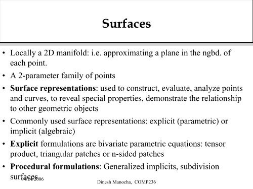
<strong>Surfaces</strong><br />
• Locally a 2D manifold: i.e. approximating a plane in the ngbd. of<br />
each point.<br />
• A 2-parameter family of points<br />
• Surface representations: à<br />
used to construct, evaluate, analyze points<br />
<strong>and</strong> curves, to reveal special properties, demonstrate the relationship<br />
to other geometric à<br />
objects<br />
• Commonly used surface representations: explicit (parametric) or<br />
implicit (algebraic)<br />
• Explicit <strong>for</strong>mulations are bivariate parametric equations: tensor<br />
product, triangular patches or n-sided patches<br />
• Procedural <strong>for</strong>mulations: Generalized implicits, subdivision<br />
surfaces<br />
Dinesh Manocha, COMP236
04/24/2006<br />
Implicit <strong>Surfaces</strong><br />
• Implicit <strong>for</strong>mulation:F(x,y,z) = 0, where F() is a polynomial in x,y<br />
<strong>and</strong> z of the <strong>for</strong>m:<br />
P<br />
aijkx i,j,k<br />
à<br />
iyjz k =0<br />
• If F() is irreducible à polynomial, the degree of the surface is: i+j+k<br />
• <strong>Geometric</strong>ally the degree refers to the maximum number of<br />
intersections any line can have the surface (assuming finite<br />
intersections)<br />
• Any rational parametric surface can be converted into algebraic<br />
(implicit) surface: implicitization<br />
Dinesh Manocha, COMP236
04/24/2006<br />
Quadric <strong>Surfaces</strong><br />
• Given as F(x,y,z) = 0, where F() is a quadratic polynomial in x,y <strong>and</strong><br />
z of the <strong>for</strong>m:<br />
Ax<br />
à<br />
2 + By2 + Cz2 +2Dxy +2Eyz +2Fxz +2Gx +2Hy +2Jz + K =0<br />
If A = B = C = -K = 1 & D = E = F = G = H = J = 0, then it produces a<br />
unit sphere at<br />
à<br />
the origin.<br />
• Also given in matrix <strong>for</strong>m as: P Q P T = 0, where P = [x y z 1] &<br />
Q =<br />
A D F G<br />
D B E H<br />
F E C J<br />
G H J K<br />
Dinesh Manocha, COMP236
04/24/2006<br />
Quadric <strong>Surfaces</strong><br />
• The coefficients of Q many have no direct physical or geometric<br />
meaning<br />
• A rigid body trans<strong>for</strong>mation, can be directly applied to Q as:<br />
à<br />
Q’ = T –1 Q [T –1 ] T<br />
à<br />
• Certain properties of the matrix of quadric equation are invariant<br />
under rigid trans<strong>for</strong>mation, including the determinants |Q| <strong>and</strong><br />
|Qu |,where Qu is the matrix corresponding to the gradient (or normal)<br />
vectors<br />
Dinesh Manocha, COMP236
04/24/2006<br />
Parametric <strong>Surfaces</strong><br />
• The most common mathematical element used to model a surface is<br />
a patch (equivalent to a segment of spline curve).<br />
• A patch is a curve-bounded collection of points whose coordinates<br />
are given àby<br />
continuous, bivariate, single-valued polynomials of the<br />
<strong>for</strong>m P(u,w) = (x y z), where:<br />
x = X(u,w) y = Y(u,w) z = Z(u,w),<br />
à<br />
where the parametric variables u <strong>and</strong> w are typically constrained to the<br />
intervals, u,w ∈<br />
[0,1].<br />
• This generates a rectangular patch, though there are other topological<br />
variations (e.g. triangular or n-sided).<br />
• Fixing the value of one of the parametric variables results in a curve<br />
on the patch in terms of the other variable. Or generate a curve net.<br />
Dinesh Manocha, COMP236
04/24/2006<br />
Parametric <strong>Surfaces</strong>: Patches<br />
• Each patch has a set of boundary conditions associated with it:<br />
four corner points (P(0,0), P(0,1), P(1,0), P(1,1)),<br />
four curves defining its edges (P(u,0), P(u,1), P(0,w), P(1,w)),<br />
tangent vectors or planes (Pu(u,w), P<br />
à<br />
w(u,w))<br />
normal vectors (Pu(u,w) X Pw(u,w)) twist vectors defined at the corner points<br />
à<br />
• In practice, composite arrays are put together or assembled to represent complex<br />
surfaces (with some appropriate continuity conditions at the boundary)<br />
• Commonly used patches: Hermite patch, Bezier patch, B-spline patch (or NURBS)<br />
Dinesh Manocha, COMP236
04/24/2006<br />
Parametric Patches<br />
• Tensor product or rectangular patches are of the <strong>for</strong>m:<br />
P<br />
P(u,w) = u,w [0,1].<br />
i,j<br />
P i,jB m i (u)Bn j (w) ∈<br />
à<br />
The number of control points is (m+1)(n+1)<br />
• Triangular patches à have triangular domain. They are of the <strong>for</strong>m:<br />
Pn<br />
nài P<br />
P(r,s,t) = r,s,t 0<br />
Pi,jr i=0 j=0<br />
isjtnàiàj , r+ s + t =1; õ<br />
It has (n+1)(n+2)/2 control points<br />
Dinesh Manocha, COMP236
04/24/2006<br />
Tensor Product Bezier Patches<br />
• Earlier work by de Casteljau (1959-63)<br />
• Later work by Bezier made them popular <strong>for</strong> CAGD<br />
• The simplest tensor product patch is a bilinear patch, based on the concept of<br />
bilinear interpolation (fitting simplest surface among 4 points)<br />
à<br />
• Bilinear Patch: Given 4 points, b 00, b 01 ,b 10 ,b 11, the patch is defined as:<br />
àP(u, w) = P1<br />
P<br />
i=0<br />
1<br />
j=0<br />
bijB1 i (u)B1j (w)<br />
or in matrix <strong>for</strong>m, it can be expressed as:<br />
[1 à u u] â b00 b01 b10 b11 ã â 1 à w<br />
w<br />
Dinesh Manocha, COMP236<br />
ã
04/24/2006<br />
Bilinear Tensor Product Bezier<br />
Patches<br />
• They are called a hyperbolic paraboloid<br />
• Consider the surface, z = xy. It is the bilinear interpolant of 4 points<br />
àâ<br />
à<br />
0<br />
0<br />
0<br />
ã , â 1<br />
0<br />
0<br />
ã , â 0<br />
1<br />
0<br />
ã , â 1<br />
1<br />
1<br />
• If we intersect with a plane parallel to the x,y plane, the resulting<br />
curve is a hyperbola. If we intersect it with a plane containing the zaxis,<br />
the resulting curve is a parabola.<br />
ã<br />
Dinesh Manocha, COMP236
04/24/2006<br />
Direct de Casteljau Algorithm<br />
• Extension of linear interpolation (or convex combination) algorithm <strong>for</strong> curves to<br />
surfaces<br />
• Given a rectangular array of points, bij, 0 ≤ i,j ≤ n <strong>and</strong> parameter value (u,w).<br />
Compute a point on a surface determined by this array of points by setting:<br />
b r,r<br />
i,j =<br />
r = 1,….,n<br />
à<br />
à<br />
[1 à u u]<br />
i,j = 0,….,n-r <strong>and</strong><br />
b n,n<br />
0,0<br />
â b rà1,rà1<br />
i,j<br />
b rà1,rà1<br />
i+1,j<br />
b 0,0<br />
i,j = b i,j<br />
b rà1,rà1<br />
i,j+1<br />
b rà1,rà1<br />
i+1,j+1<br />
is the point with parameter values (u,w) on the surface<br />
ã<br />
Dinesh Manocha, COMP236<br />
â 1 à w<br />
w<br />
ã
04/24/2006<br />
Direct de Casteljau Algorithm<br />
• The net of b ij, is called the Bezier net or the control net.<br />
• Tensor product <strong>for</strong>mulation: A surface is the locus of a curve that is<br />
moving thru space <strong>and</strong> thereby changing its shape<br />
• The same àsurface<br />
can also be represented using Bernstein basis as:<br />
P(u, w) =<br />
à<br />
Pn<br />
i=0<br />
Pn<br />
j=0<br />
bijB n<br />
i (u)Bnj<br />
(w)<br />
• de Casteljau’s be easily extended when the control points along u <strong>and</strong><br />
w directions are different (say m X n)<br />
– Apply the recursive <strong>for</strong>mulation till b is computed, where<br />
k = min(m,n)<br />
k,k<br />
i,j<br />
– After that use the univariate de Casteljau’s algorithm<br />
Dinesh Manocha, COMP236
• Affine invariance<br />
04/24/2006<br />
Properties of Bezier Patches<br />
• Convex hull property<br />
• Boundary curves: are Bezier curves<br />
• Variation àdimishing<br />
property: Not clear whether it holds <strong>for</strong> surfaces<br />
– Easy to come with an counter example<br />
à<br />
Dinesh Manocha, COMP236
04/24/2006<br />
Degree Elevation<br />
• Goal: To raise the degree from (m,n) to (m+1,n)<br />
• Compute new coefficients, b , such that the surface can be<br />
expressed as:<br />
1,0<br />
i,j<br />
à<br />
P(u, w) =<br />
à<br />
• The n+1 terms in square brackets represent n+1 univariate degree<br />
elevation<br />
P â n Pm+1<br />
(1,0)<br />
j=0 i=0 b ij Bm+1<br />
i (u) ã B n j (w)<br />
• The new control points can be computed, by using the univariate<br />
<strong>for</strong>mula:<br />
b 1,0<br />
i,j = i i<br />
(1 à )bi,j + bià1,j<br />
m+1 m+1<br />
è i =0,...,m+1<br />
j =0,...n<br />
Dinesh Manocha, COMP236
04/24/2006<br />
Derivatives<br />
• Goal: To compute partials along u or w directions<br />
• A partial derivative is the tangent vector of an isoparametric curve:<br />
P(u, w)<br />
à<br />
=<br />
• It can be expressed as:<br />
à<br />
Pn<br />
â<br />
∂<br />
∂<br />
j=0 ∂u<br />
∂u<br />
P<br />
∂ Pn<br />
P(u, w) =m j=0<br />
∂u<br />
P<br />
i=0<br />
where<br />
Dinesh Manocha, COMP236<br />
m<br />
i=0<br />
bijB m i (u)ãB n j (w)<br />
mà1 (1,0) Δ bijB mà1<br />
i (u)B n j (w)<br />
Δ 1,0 b i,j = b i+1,j à b i,j<br />
,
04/24/2006<br />
Trimmed Patches<br />
• Arise in applications involving surface intersections, visibility<br />
(silhouettes), illumination etc.<br />
• The domain is irregular<br />
• Boundary àor<br />
trimming curves are used to delimit a subset of points on<br />
the patch<br />
• In most applications, à<br />
trimming curves correspond to high degree<br />
algebraic curves<br />
– Evaluate points on these curves using numerical methods<br />
– Fit spline curve(s) to these points<br />
• Trimmed domain is represented using piecewise spline curves<br />
• Point Classification:Check whether a point is in the trimmed domain,<br />
compute number of intersections with a line<br />
Dinesh Manocha, COMP236


