Adaptive Frustum Tracing for Interactive Sound Propagation

c○2009 IEEE. Reprinted, with permission, from IEEE TRANSACTION ON VISUALIZATION AND COMPUTER GRAPHICS, VOL. 14, NO. 6, NOVEMBER/DECEMBER 2008
AD-Frustum: Adaptive Frustum Tracing for Interactive Sound
Propagation
Anish Chandak, Christian Lauterbach, Micah Taylor, Zhimin Ren, and Dinesh Manocha, Member, IEEE
Abstract—We present an interactive algorithm to compute sound propagation paths for transmission, specular reflection and edge
diffraction in complex scenes. Our formulation uses an adaptive frustum representation that is automatically sub-divided to accurately
compute intersections with the scene primitives. We describe a simple and fast algorithm to approximate the visible surface for each
frustum and generate new frusta based on specular reflection and edge diffraction. Our approach is applicable to all triangulated
models and we demonstrate its performance on architectural and outdoor models with tens or hundreds of thousands of triangles and
moving objects. In practice, our algorithm can perform geometric sound propagation in complex scenes at 4-20 frames per second
on a multi-core PC.
Index Terms—Sound propagation, interactive system, auralization
1 INTRODUCTION
Sound simulation and spatialized audio rendering can significantly enhance
the realism and sense of immersion in interactive virtual environments.
They are useful for computer-aided acoustic modeling,
multi-sensory visualization, and training systems. Spatial sound can
be used for development of auditory displays or provide auditory cues
for evaluating complex datasets [22, 33].
A key component of 3D audio rendering is interactive sound propagation
that simulates sound waves as they reflect or diffract off objects
in the virtual environment. One of the main challenges in sound rendering
is handling complex datasets at interactive rates. Current visual
rendering systems can render datasets composed of millions of primitives
at real-time rates (i.e. 10-30 fps) on commodity desktop systems.
On the other hand, interactive sound rendering algorithms are only
limited to scenes with a few thousand triangles. Therefore, most interactive
applications typically use precomputed, static sound effects
based on fixed models of propagation.
In this paper, we address the problem of interactive sound propagation
in complex datasets from point sources. The exact solution to
modeling propagation is based on solving the Helmholtz-Kirchhoff integration
equation. The numerical methods to solve this equation tend
to be compute and storage intensive. As a result, fast algorithms for
complex scenes mostly use geometric methods that propagate sound
based on rectilinear propagation of waves and can accurately model
transmission, early reflection and edge diffraction [11]. The most accurate
geometric approaches are based on exact beam or pyramid tracing,
which keep track of the exact shape of the volumetric waves as
they propagate through the scene. In practice, these approaches are
mainly limited to static scenes and may not be able to handle complex
scenes with curved surfaces at interactive rates. On the other hand,
approximate geometric methods based on path-tracing or ray-frustum
tracing can handle complex, dynamic environments, but may need a
very large number of samples to overcome aliasing errors.
Main results: We present a novel volumetric tracing approach
that can generate propagation paths for early specular reflections and
edge diffraction by adapting to the scene primitives. Our approach is
• Anish Chandak, E-mail: achandak@cs.unc.edu.
• Christian Lauterbach, E-mail: cl@cs.unc.edu.
• Micah Taylor, E-mail: taylormt@cs.unc.edu.
• Zhimin Ren, E-mail: zren@cs.unc.edu.
• Dinesh Manocha, E-mail: dm@cs.unc.edu.
• Project Webpage: http://gamma.cs.unc.edu/SOUND
Manuscript received 31 March 2008; accepted 1 August 2008; posted online
19 October 2008; mailed on 13 October 2008.
For information on obtaining reprints of this article, please send
e-mailto:tvcg@computer.org.
general and can handle all triangulated models with moving objects.
The underlying formulation uses a simple adaptive representation that
augments a 4-sided frustum [19] with a quadtree and adaptively generates
sub-frusta. We exploit the representation to perform fast intersection
and visibility computations with scene primitives. As compared
to prior adaptive algorithms for sound propagation, our approach provides
an automatic balance between accuracy and interactivity to generate
plausible sound rendering in complex scenes. Some novel aspects
of our work include:
1. AD-Frustum: We present a simple representation to adaptively
generate 4-sided frusta to accurately compute propagation paths. Each
sub-frustum represents a volume corresponding to a bundle of rays.
We use ray-coherence techniques to accelerate intersection computations
with the corner rays. The algorithm uses an area subdivision
method to compute an approximation of the visible surface for each
frustum.
2. Edge-diffraction: We present an efficient algorithm to perform
edge diffraction on AD-Frustum based on the Uniform Theory
of Diffraction [15, 37]. These include efficient techniques to compute
the shape of diffraction frustum and the actual contribution that the
diffraction makes at the listener.
3. Handling complex scenes: We use bounding volume hierarchies
(BVHs) to accelerate the intersection computations with AD-Frusta in
complex, dynamic scenes. We present techniques to bound the maximum
subdivision within each AD-Frustum based on scene complexity
and thereby control the overall accuracy of propagation by computing
all the important contributions.
We have applied our algorithm for interactive sound propagation in
complex and dynamic scenes corresponding to architectural models,
outdoor scenes, and game environments. In practice, our algorithm
can accurately compute early sound propagation paths with up to 4-5
reflections at 4-20 frames per second on scenes with hundreds of thousands
of polygons on a multi-core PC. Our preliminary comparisons
indicate that propagation based on AD-Frusta can offer considerable
speedups over prior geometric propagation algorithms. We also evaluate
the accuracy of our algorithm by comparing the impulse responses
with an industrial strength implementation of an image source method.
Organization: The rest of the paper is organized in the following
manner. We briefly survey related work on geometric sound propagation
and interactive sound rendering in Section 2. Section 3 describes
the AD-Frustum representation and intersection computations.
We present algorithms to enumerate propagation paths in Section 4
and highlight techniques to handle complex environments in Section
5. We describe the overall performance and accuracy in Section 6.

Update Sources
Update Listener
Update BVH
Query direct
contribution
Primary Frustum
AD−Frustum
Intersection
with BVH
{Δ1,..., ΔΚ}
triangles
Intersection
with
triangles
Visible Surface Approximation
Secondary Frustum
Specular Reflection
+
Edge Diffraction
AD−Frustum (quadtree updated)
Enumerate Propagation Paths
Constribution to
the listener
Audio
Rendering
Query direct
contribution
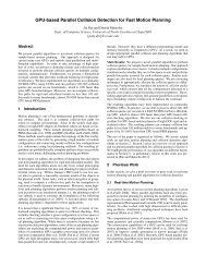
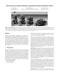
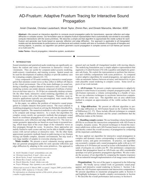
Fig. 1. Overview of our algorithm: AD-Frusta are generated from sound sources (primary frusta) and by reflection and diffraction (secondary frusta)
from the scene primitives. Approximate visible surfaces are then computed for each frustum (quadtree update). Next, each updated frustum checks
if the listener lies inside it and is visible. If visible, its contributions are registered with the audio rendering system. The audio rendering system
queries the direct contribution of a sound source every time it renders its audio block.
2 PREVIOUS WORK
The two main approaches to sound propagation are numerical methods
and geometric approaches [11, 32]. In practice, the numerical
solutions are too slow for interactive applications or dynamic scenes.
In this section, we focus on geometric propagation techniques, which
are primarily used to model early specular reflection and diffraction
paths. Recently, techniques based on acoustic radiosity have also been
developed to handle diffuse reflections for simple indoor scenes. At a
broad level, the geometric propagation methods can be classified into
ray-based or particle-based tracing, image source methods, and volumetric
tracing.
Ray-based or Particle-based Techniques: Some of the earliest
methods for geometric sound propagation are based on tracing
sampled-rays [16] or sound-particles (phonons) [14, 2, 6, 23] from a
source to the listener. Recent improvements, including optimized hierarchies
and exploiting ray-coherence, make it possible for ray-based
and particle-based methods to handle complex, dynamic scenes on
commodity hardware [39] or handle massive models [20]. However,
due to discrete sampling of the space, these methods have to trace large
number of paths or particles to avoid aliasing artifacts.
Image Source Methods: These methods are the easiest and most
popular for computing specular reflections [1, 5]. They compute virtual
sources from a sound source recursively for every reflection and
can have exponential complexity in the number of reflections. They
can guarantee all specular paths up to a given order. However, they
can only handle simple static scenes or very low order of reflections at
interactive rates [17]. Many hybrid combinations [4] of ray-based and
image source methods have also been proposed and used in commercial
room acoustics prediction softwares (e.g. ODEON).
Volumetric Methods: The volumetric methods trace pyramidal or
volumetric beams to compute an accurate geometric solution. These
include beam tracing that has been used for specular reflection and
edge diffraction for interactive sound propagation [10, 17, 37, 9]. The
results of beam tracing can be used to guide sampling for path tracing
[10]. However, the underlying complexity of beam tracing makes it
hard to handle complex models. Other volumetric tracing methods are
based on triangular pyramids [8], ray-beams [25], ray-frusta [19], as
well as methods developed for visual rendering [12].
Interactive Sound Propagation: Various approaches have been
proposed to improve the performance of acoustic simulation or handle
complex scenarios. These include model simplification algorithms
[13], use of scattering filters [36], and reducing the number of active
sound sources by perceptual culling or sampling [38, 40]. These techniques
are complementary to our approach and can be combined to
handle scenarios with multiple sound sources or highly tessellated objects
in the scene.
3 ADAPTIVE VOLUME TRACING
Our goal is to perform interactive geometric sound propagation in
complex and dynamic scenes. We mainly focus on computing paths
that combine transmission, specular reflection, and edge diffraction up
to a user-specified criterion from each source to the receiver. Given
the underlying complexity of exact approaches, we present an approximate
volumetric tracing algorithm. Fig. 1 gives a top level view of
our algorithm. We start by shooting frusta from the sound sources.
A frustum traverses the scene hierarchy and finds a list of potentially
intersecting triangles. These triangles are intersected with the frustum
and the frustum is adaptively sub-divided into sub-frusta. The
sub-frusta approximate which triangles are visible to the frustum. The
sub-frusta are subsequently reflected and diffracted to generate more
frusta, which in turn are traversed. Also, if the listener is inside a
frustum and visible, the contribution is registered for use during audio
rendering stage.
Our approach builds on using a ray-frustum for volumetric tracing
[19]. We trace the paths from the source to the receivers by tracing
a sequence of ray-frusta. Each ray-frustum is a simple 4-sided frustum,
represented as a convex combination of four corner rays. Instead
of computing an exact intersection of the frusta with a primitive,
ray-frustum tracing performs discrete clipping by intersecting a fixed
number of rays for each frustum. This approach can handle complex,
dynamic scenes, but has the following limitations:
• The formulation uses uniformly spaced samples inside each frustum
for fast intersection computations. Using a high sampling
resolution can significantly increase the number of traced frusta.
• The approach cannot adapt to the scene complexity efficiently.
In order to overcome these limitations, we propose an adaptive frustum
representation, AD-Frustum. Our goal is to retain the performance
benefits of the original frustum formulation, but increase the accuracy
of the simulation by adaptively varying the resolution. Various components
of our algorithm are shown in Fig. 1.
3.1 AD-Frustum
AD-Frustum is a hierarchical representation of the subdivision of a
frustum. We augment a 4-sided frustum with a quadtree structure to
keep track of its subdivision and maintain the correct depth information,
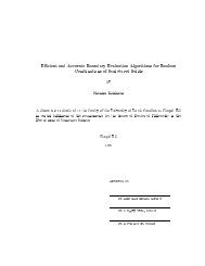
as shown in Fig. 2. Each leaf node of the quadtree represents the
finest level sub-frustum that is used for volumetric tracing. An intermediate
node in the quadtree corresponds to the parent frustum or an
internal frustum. We adaptively refine the quadtree in order to perform
accurate intersection computations with the primitives in the scene and
generate new frusta based on reflections and diffraction.
Representation: Each AD-Frustum is represented using an apex
and a quadtree. Each 2D node of the quadtree includes: (a) corner
rays of the sub-frustum that define the extent of each sub-frustum;
(b) intersection status corresponding to completely-inside, partiallyintersecting
with some primitive, or completely-outside of all scene
primitives; (c) intersection depth, and primitive id to track the depth
value of the closest primitive; (d) list of diffracting edges to support
diffraction calculations. We also associate a maximum-subdivision
depth parameter with each AD-Frustum that corresponds to the maximum
depth of the quadtree.
3.2 Intersection Tests
The AD-Frusta are used for volumetric tracing and enumerating the
propagation paths. The main operation is computing their intersection
with the scene primitives and computing reflection and diffraction

c○2009 IEEE. Reprinted, with permission, from IEEE TRANSACTION ON VISUALIZATION AND COMPUTER GRAPHICS, VOL. 14, NO. 6, NOVEMBER/DECEMBER 2008
A P
(a) (b)
Fig. 2. AD-Frustum Representation: (a) A frustum, represented by convex
combination of four corner rays and apex A. (b) A hierarchically
divided adaptive frustum. It is augmented with a quadtree structure,
where P is the 2D plane of quadtree. We use two sets of colors to
show different nodes. Each node stores auxiliary information about corresponding
sub-frusta.
frusta. The scene is represented using a bounding volume hierarchy
(BVH) of axis-aligned bounding boxes (AABBs). The leaf nodes of
the BVH are triangle primitives and the intermediate nodes represent
an AABB. For dynamic scenes, the BVH is updated at each frame
[39, 21, 43]. Given an AD-Frustum, we traverse the BVH from the
root node to perform these tests.
Intersection with AABBs: The intersection of an AD-Frustum
with an AABB is performed by intersecting the four corner rays of
the root node of the quadtree with the AABB, as described in [26]. If
an AABB partially or fully overlaps with the frustum, we apply the algorithm
recursively to the children of the AABB. The quadtree is not
modified during this traversal.
Intersection with primitives: As a frustum traverses the BVH,
we compute intersections with each triangle corresponding to the leaf
nodes of the BVH. We only perform these tests to classify the node as
completely-inside, completely-outside or partially-intersecting. This
is illustrated in Fig. 3, where we show the completely-outside regions
in green and completely-inside regions in orange. This intersection
test can be performed efficiently by using the Plücker coordinate
representation [31] for the triangle edges and four corner rays. The
Plücker coordinate representation efficiently determines, based on an
assumed orientation of edges, whether the sub-frustum is completely
inside, outside or partially intersecting the primitive. This test is conservative
and may conclude that a node is partially intersecting, even
if it is completely-outside. If the frustum is classified as partiallyintersecting
with the primitives, we sub-divide that quadtree node,
generate four new sub-frusta, and perform the intersection test recursively.
The maximum-subdivision depth parameter imposes a bound
on the depth of the quadtree. Each leaf node of the quadtree is classified
as completely-outside or completely-inside.
3.3 Visible Surface Approximation
A key component of the traversal algorithm is the computation of the
visible primitives associated with each leaf node sub-frustum. We use
an area-subdivision technique, similar to classic Warnock’s algorithm
[41], to compute the visible primitives. Our algorithm associates intersection
depth values of four corner rays with each leaf node of the
quadtree as well as the id of the corresponding triangle. Moreover,
we compute the minimum and maximum depth for each intermediate
node of the triangle, that represents the extent of triangles that partially
overlap with its frustum. The depth information of all the nodes
is updated whenever we perform intersection computations with a new
triangle primitive.
In order to highlight the basic subdivision algorithm, we consider
the case of two triangles in the scene shown as red and blue in Fig. 3.
In this example, the projections of the triangles on the quadtree plane
overlap. We illustrate different cases that can arise based on the relative
ordering and orientation of two triangles. The basic operation
compares the depths of corner rays associated with the frustum and
updates the node with the depth of the closer ray (as shown in Fig.
3(a)). If we cannot resolve the closest depth (see Fig. 3(d)), we apply
the algorithm recursively to its children (shown in orange). Fig.
3(b) shows the comparison between a partially-intersecting node with
a completely-inside node. If the completely-inside node is closer, i.e.,
all the corner rays of the completely-inside node are closer than the
minimum depth of the corner rays of the partially-intersecting node,
then the quadtree is updated with the completely-inside node. Otherwise,
we apply the algorithm recursively to their children as in Fig.
3(e). Lastly, in Fig. 3(c), both the nodes are partially-intersecting and
we apply the algorithm recursively on their children.
This approach can be easily generalized to handle all the triangles
that overlap with an AD-Frustum. At any stage, the algorithm maintains
the depth values based on intersection with all the primitives traversed
so far. As we perform intersection computations with a new
primitive, we update the intersection depth values by comparing the
previous values stored in the quadtree. The accuracy of our algorithm
is governed by the resolution of the leaf nodes of the quadtree, which
is based on the maximum-subdivision depth parameter associated with
each AD-Frustum.
3.4 Nodes Reduction
We perform an optimization step to reduce the number of frusta. This
step is performed in a bottom up manner, after AD-Frustum finishes
the scene traversal. We look at the children of a node. Since, each
child shares atleast one corner-ray with its siblings, we compare the
depths of these corner-rays. Based on the difference in depth values,
the normals of the surfaces the sub-frustum intersects, and the acoustic
properties of those surfaces we collapse the children nodes into the
parent node. Thus, we can easily combine the children nodes in the
quadtree that hit the same plane with similar acoustic properties. Such
an approach can also be used to combine children nodes that intersect
slightly different surfaces.
4 ENUMERATING PROPAGATION PATHS
In the previous section, we described the AD-Frustum representation
and presented an efficient algorithm to compute its intersection and
visibility with the scene primitives. In this section, we present algorithms
to trace the frusta through the scene, and compute reflection
and diffraction frusta. We start the simulation by computing initial
frusta around a sound source in quasi-uniform fashion [27] and perform
adaptive subdivision based on the intersection tests. Ultimately,
the sub-frusta corresponding to the leaf nodes of the quadtree are used
to compute reflection and diffraction frusta.
Specular Reflections: Once a frustum has completely traced a
scene, we consider all the leaf nodes within its quadtree and compute
a reflection frustum for all completely-intersecting leaf nodes. The
corner rays of sub-frustum associated with the leaf nodes are reflected
(see Fig. 5) at the primitive hit by that sub-frustum. The convex combination
of the reflected corner rays creates the parent frustum for the
reflection AD-Frustum.
4.1 Edge Diffraction
Diffraction happens when a sound wave hits an object whose size is
the same order of magnitude as its wavelength, causing the wave to
scatter. Our formulation of diffraction is based on the uniform theory
of diffraction (UTD) [15], which predicts that a sound wave hitting an
edge between the primitives is scattered in a cone. The half-angle of
the cone is determined by the angle that the ray hits the edge. The basic
ray-frustum tracing algorithm can compute edge diffraction based on
UTD [34]. This involves identifying diffraction edges as part of a
pre-process and computing diffraction paths using frusta tracing. In
this section, we extend the approach described in [34] to handle AD-
Frusta.
Finding diffracting edges: In a given scene, only a subset of the
edges are diffraction edges. For example, any planar rectangle is represented
by two triangles sharing an edge, but that edge cannot result in
diffraction. Most edges in a model are shared by at least two triangles.
As part of a pre-computation step, we represent the adjacency information
using an edge-based data structure that associates all edges that
can result in diffraction with its incident triangles. As part of the tracing
algorithm, we compute all triangles that intersect a sub-frustum.
Next, we check whether the sub-frustum intersects any of the edges
of that triangle and based on that update the list of diffracting edges

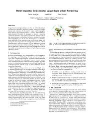
(a) (b) (c) (d) (e)
Fig. 3. Visibility computation based on area subdivision: We highlight different cases that arise as we resolve visibility between two triangle
primitives (shown in red and blue) from the apex of the frustum. In cases (a)-(b) the quadtree is refined based on the intersection depth associated
with the outermost frustum and compared with the triangles. However, in cases (c)-(e) the outermost frustum has to be sub-divided into sub-frusta
and each of them is compared separately.
Fig. 4. Generating a diffraction frustum from an edge. The resulting
wedge is shown as red and we show the generation of diffraction
shadow frustum from the original sub-frustum. Note that the origin for
the frustum is not just the edge, but the whole area of the sub-frustum
that overlaps the edge.
for that sub-frustum. We perform these tests efficiently using Plücker
coordinates.
Computing Diffraction Frusta: Our adaptive diffraction approach
is similar to the diffraction formulation described in [34, 37]. There
are two main problems that arise in simulating edge diffraction using
frusta: first, finding the shape of the new frustum that corresponds
to the real diffraction as predicted by the UTD; second, computing
the actual contribution that the diffraction makes to the sound at the
listener.
Given a diffraction edge, we clip the sub-frustum against the edge
to find the interval along the edge that it intersects. The diffraction
cone originates from the respective part of the edge and its orientation
and shape are predicted by the UTD based on the angle of the edge.
The angle is computed from the triangles incident to the edge. Notice
that we perform an approximation similar to [37] in that we ignore the
non-‘shadow’ part of the diffraction. As part of frustum tracing, we
ensure that the origin of the diffraction frustum is not limited to lie on
the edge, but is chosen as the whole area of the frustum that overlaps
the edge (see Fig. 4 for illustration). We compute this area by clipping
the quadrilateral defined by the intersection of the frustum with the triangle’s
plane against the triangle edge. This computation extends the
frustum shape beyond the actual diffraction field originating from the
edge. This has the important practical advantage that it will include
the direct contribution of the original frustum for parts of the frustum
that do not overlap with the triangle. As a result, this formulation actually
adds back direct contributions that would have been lost due to
the discrete nature of the frustum representation. One special case occurs
if just one corner of the frustum is inside the triangle, since in
that case the clipped frustum has five edges. We handle this case by
using a conservative bounding frustum and performing an additional
check for inclusion when we compute all the contributions to the listener.
Note that UTD is valid only for scenes with long edges, like the
outdoor city scene or large walls and doors of architecture models. We
therefore perform edge-diffraction on such models.
4.2 Contributions to the Listener
For the specular reflections the actual contribution of a frustum is determined
by finding a path inside all the frusta from the sound source
to the listener. In case of diffraction, we have to ensure that the subfrustum
is actually in the real diffraction shadow part of the frustum.
There are three distinct possibilities: first, the sub-frustum can be part
of the direct contribution as described above. In that case, the contribution
is simply computed like a direct one. The second case is that
the sub-frustum is not a direct one, but also not inside the diffraction
cone, i.e. inside the conservative bounding frustum. In that case, it
can be safely ignored. Finally, if the listener’s location is inside the
diffraction frustum, we can compute the exact path due to all diffraction
events. The UTD formulation predicts the intensity of the sound
field inside the diffraction cone, which depends on several variables,
but most importantly the angle to the line of visibility (see [34, 37] for
more details). For the frustum representation, the equation can either
be evaluated while computing the exact path, or per sub-frustum, i.e.
by discretizing the equation. In our formulation, we chose the latter
such that the contribution can be evaluated very quickly per frustum,
with a slight impact on the exact timing of the diffraction.
5 COMPLEX SCENES
In this section, we give a brief overview of how to govern the accuracy
of our algorithm for complex scenes. The complexity of the
AD-Frustum tracing algorithm described in Sections 3 and 4 varies
as a function of the maximum-subdivision depth parameter associated
with each AD-Frustum. A higher value of this parameter results in a
finer subdivision of the quadtree and improves the accuracy of the intersection
and volumetric tracing algorithms (see Fig. 5). At the same
time, the number of leaf nodes can potentially increase as an exponential
function of this parameter and significantly increase the number of
traced frusta through the scene. Here, we present techniques for automatic
computation of the depth parameter for each AD-Frustum. We
consider two different scenarios: capturing the contributions from all
important objects in the scene and constant frame-rate rendering.
Our basic algorithm is applicable to all triangulated models. We do
not make any assumptions about the connectivity of the triangles and
can handle all polygonal soup datasets. Many times, a scene consists
of objects that are represented using connected triangles. In the context
of this paper, an object corresponds to a collection of triangles that are
very close (or connected) to each other.
5.1 Maximum-subdivision depth computation
One of the main challenges is to ensure that our algorithm doesn’t
miss the important contributions in terms of specular reflections and
diffraction. We take into account some of the characteristics of geometric
sound propagation in characterizing the importance of different
objects. For example, many experimental observations have suggested
that low-resolution geometric models are more useful for specular reflections
[13, 36]. Similarly, small objects in the scene only have
significant impact at high frequencies and can be excluded from the
models in the presence of other significant sources of reflection and
diffraction [10]. Based on these characterizations, we pre-compute geometric
simplifications of highly tessellated small objects and assign
an importance function to each object based on its size and material
properties.
Given an object (O) with its importance function, our goal is to ensure
that the approximate frustum-intersection algorithm doesn’t miss
contributions from that object. Given a frustum with its apex (A) and

c○2009 IEEE. Reprinted, with permission, from IEEE TRANSACTION ON VISUALIZATION AND COMPUTER GRAPHICS, VOL. 14, NO. 6, NOVEMBER/DECEMBER 2008
(a) (b) (c) (d) (e) (f)
Fig. 5. Beam tracing vs. uniform frustum tracing vs. adaptive frustum tracing: We show the relative accuracy of three different algorithm in this
simple 2D model with only first-order reflections. (a) Reflected beams generated using exact beam tracing. (b)-(c) Reflected frusta generated with
uniform frustum tracing for increased sampling: 2 2 samples per frustum and 2 4 samples per frustum. Uniform frustum tracing generates uniform
number of samples in each frustum, independent of scene complexity. (d)-(e) Reflected frusta generated using AD-Frustum. We highlight the
accuracy of the algorithm by using the values of 2 and 4 for maximum-subdivision depth parameter. (f) An augmented binary tree for the 2D case
(equivalent to a quadtree in 3D) showing the adaptive frusta. Note that the adaptive algorithm only generates more frusta in the regions where the
input primitives have a high curvature and reduces the propagation error.
the plane of its quadtree (P), we compute a perspective projection of
the bounding box of O on the P. Let’s denote the projection on P as
o. Based on the size of o, we compute a bound on the size of leaf
nodes of the quadtree such that the squares corresponding to the leaf
nodes are inside o. If O has a high importance values attached to it,
we ensure multiple leaf nodes of the quadtree are contained in o. We
repeat this computation for all objects with high importance value in
the scene. The maximum-subdivision depth parameter for that frustum
is computed by considering the minimum size of the leaf nodes
of the quadtree over all objects. Since we use a bounding box of O to
compute the projection, our algorithm tends to be conservative.
5.2 Constant frame rate rendering
In order to achieve target frame rate, we can bound the number of
frusta that are traced through the scene. We first estimate the number
of frustum that our algorithm can trace per second based on scene
complexity, number of dynamic objects and sources. Given a bound
on maximum number of frusta traced per second, we adjust the number
of primary frusta that are traced from each source. Moreover, we
use a larger value of the maximum depth parameter for the first few
reflections and decrease this value for higher order reflections. We
compute the first few reflections with higher accuracy by performing
more adaptive subdivisions. We also perform adaptive subdivisions
of a frustum based on its propagated distance. In this manner, our
algorithm would compute more contributions from large objects in
the scene, and tend to ignore contributions from relatively small objects
that are not close to the source or the receiver. We can further
improve the performance by using dynamic sorting and culling algorithms
along with perceptual metrics [38].
6 IMPLEMENTATION AND RESULTS
In this section, we highlight the performance of our algorithm on different
benchmarks, describe our audio rendering pipeline, and analyze
its accuracy. Our simulations were run on a 2.66 GHz Intel Core 2
Duo machine with 2GB of memory.
6.1 Performance Results
We perform geometric sound propagation using adaptive frustum tracing
on many benchmarks. The complexity of our benchmarks ranges
from a few hundred triangles to almost a million triangles. The performance
results for adaptive frustum tracing and complexity of benchmarks
are summarized in Table 1. These results are generated for a
maximum sub-division depth of 3. Further, the extent of dynamism in
these benchmarks is shown in associated video. In Fig. 7, we show
how the computation time for our approach and the number of frusta
traced scale as we increase the maximum sub-division depth of AD-
Frusta. Also, our algorithm scales well with the number of cores as
shown in Fig. 8. The comparison of our approach with uniform frustum
tracing [19] is given in Table 2. We chose a sampling resolution of
2 3 × 2 3 for uniform frustum tracing and maximum sub-division depth
of 3 for adaptive frustum tracing for the purposes of comparisons.
Model Complexity Results (7 threads)
#Δs diffraction #frusta time
Theater 54 NO 56K 33.3 ms
Factory 174 NO 40K 27.3 ms
Game 14K NO 206K 273.3 ms
Sibenik 71K NO 198K 598.6 ms
City 78K YES 80K 206.2 ms
Soda Hall 1.5M YES 108K 373.3 ms
Table 1. This table summarizes the performance of our system on six
benchmarks. The complexity of a model is given by the number of triangles.
We perform edge diffraction in two models and specular reflection
in all. We use a value of 3 for the maximum sub-division depth for these
timings. The results are computed for up to 4 orders of reflection.
log(Time (msecs))
log(#Frustua)
10
8
6
4
Theater
Factory
Game
Sibenik
City
Soda Hall
2
2 3 4 5
Maximum Sub−division depth
16
14
12
10
Theater
Factory
Game
Sibenik
City
Soda Hall
2 3 4 5
Maximum Sub−division depth
Fig. 7. This figure shows the effect of increasing the maximum subdivision
depth of adaptive frustum tracing on the overall computation
time of the simulation and the number of total frusta traced. Different
colors are used for different benchmarks.
6.2 Audio Rendering
Audio rendering is the process of generating the final audio signal in
an application. In our case, it corresponds to the convolution of the
filter generated by sound propagation simulation with the input audio
to produce the final sound at the receiver. In this section, we outline
an audio rendering pipeline that can be integrated with our geometric
propagation approach to perform interactive audio rendering for
scenes with moving sources, moving listener, and dynamic objects.
The two main methods for performing interactive audio rendering
are “direct room impulse response rendering” and “parametric room

(a) (b) (c) (d)
Fig. 6. Different Benchmarks: (a) Game Model with low geometric complexity. It has dynamic objects and a moving listener. (b) Sibenik Cathedral,
a complex architectural model with a lot of details and curved geometry. It consists of moving source and listener, and a door that opens and closes.
(c) City Scene with many moving cars (dynamic objects) and tall buildings which cause edge diffraction. It has a moving sound source, a static
sound source, and a listener. (d) Soda Hall, a complex architectural model with multiple floors. The dimensions of a room are dynamically modified
and the sound propagation paths recomputed for this new room using AD-Frusta. This scenario demonstrates the potential of our approach for
conceptual acoustic design.
Speedup
7
6
5
4
3
2
Theater
Factory
Game
Sibenik
City
Soda Hall
1
1 2 3 4 5 6 7
Number of Cores
Fig. 8. This figure shows that our algorithm scales well with the number
of cores. It makes our approach favorable for parallel and many-core
platforms. Reflections for up to 4th order were computed and larger of
maximum sub-division depths similar to those in Table 3 were used.
Model Frusta traced Frusta Time
UFT AFT Gain Gain
Theater 404K 56K 7.2 6.1
Factory 288K 40K 7.2 5.7
Game 2330K 206K 11.3 9.0
Sibenik 6566K 198K 33.2 21.9
City 377K 78K 4.9 5.2
Soda Hall 773K 108K 7.2 9.8
Table 2. This table presents a preliminary comparison of the number of
frusta traced and time taken by Adaptive Frustum Tracing and Uniform
Frustum Tracing [19] for results of similar accuracy. Our adaptive frustum
formulation significantly improves the performance as compared to
prior approaches.
impulse response rendering” [29]. In “direct room impulse response
rendering”, impulse responses are pre-computed at some fixed listener
locations. Next, the impulse response at some arbitrary listener position
is computed by interpolating the impulse responses at nearby
fixed listener locations. Such a rendering method is not very suitable
when the source is moving or the scene geometry is changing.
“Parametric room impulse response rendering” uses parameters like
reflection path to the listener, materials of the objects in reflection path
etc. to perform interactive audio rendering. However, in this case it
is important that the underlying geometric propagation system is able
to update these parameters at very high update rates. Sandvad [28]
suggests that update rates above 10 Hz should be used. In the DIVA
system [29], an update rate of 20 Hz is used to generate artifact free
audio rendering for dynamic scenes. We also use similar audio rendering
techniques. Table 3 shows that we can update parameters at
a high rate with maximum sub-division depth of 2 on a single core,
as required by “Parametric room impulse response rendering”. Similar
update rates for a sub-division depth of 3 on a single core can be
achieved by decreasing the order of reflection or by updating the low
order reflections more frequently than higher order reflections (see Ta-
ble 3). Furthermore, we need to interpolate the parameters between
the updates, as suggested in [42, 35], to minimize the artifacts due to
the changing impulse responses. In order to demonstrate the accuracy
of our propagation algorithm, we perform audio rendering offline in
some benchmarks. Also, the impulse responses used to generate the
final rendered audio contain only early specular reflections and no late
reverberation. This is done so it is easy to evaluate the effect of early
reflections computed by our adaptive frustum tracing algorithm. Late
reverberations can be computed as a pre-processing step [29] and can
improve the audio quality.
Order of Reflection Maximum
Model Tris (Running time in msec) sub-division
1st 2nd 3rd 4th depth
Theater 54
4.7
24
8.0
77
16.0
201
30.0
462
2
4
Factory 174
3.3
18
6.7
64
12.7
178
24.7
406
2
4
Game Scene 14K
20
51
46
167
120
469
270
1134
2
3
Sibenik 71K
34
67
83
236
250
864
694
2736
2
3
City 72K
6.7 12 23 44 2
Soda Hall 1.5M
18 38 85 174 3
21 38 98 229 2
35 102 297 723 3
Table 3. This table shows the performance of adaptive frustum tracing
on a single core for different maximum sub-division depths. The timings
are further broken down according to order of reflection. Our propagation
algorithm achieves interactive performance for most benchmarks.
6.3 Accuracy and Validation
Our approach is an approximate volume tracing approach and we
can control its accuracy by varying the maximum-subdivision depth
of each AD-Frustum. In order to evaluate the accuracy of propagation
paths, we compare the impulse responses computed by our algorithm
with other geometric propagation methods. We are not aware
of any public or commercial implementation of beam tracing which
can handle complex scenes with dynamic objects highlighted in Table
1. Rather, we use an industry strength implementation of image
source method available as part of CATT-Acoustic TM software.
We compare our results for specular reflection on various benchmarks
available with CATT software (see Fig. 9 and Fig. 10). The results
show that our method gives more accurate results with higher maximum
sub-division depths.
7 ANALYSIS AND COMPARISON
In this section, we analyze the performance of our algorithm and compare
it with other geometric propagation techniques. The running time
of our algorithm is governed by three main factors: model complexity,

c○2009 IEEE. Reprinted, with permission, from IEEE TRANSACTION ON VISUALIZATION AND COMPUTER GRAPHICS, VOL. 14, NO. 6, NOVEMBER/DECEMBER 2008
amplitude
Adaptve Volume Tracing (Source=S1, Listener=L1, Subdivision=2)
0.9
0.8
0.7
0.6
0.5
0.4
0.3
0.2
0.1
0
0 2000 4000 6000 8000 10000
time
(c) 23 contributions
(a) Theater benchmark
amplitude
Adaptve Volume Tracing (Source=S1, Listener=L1, Subdivision=4)
0.9
0.8
0.7
0.6
0.5
0.4
0.3
0.2
0.1
0
0 2000 4000 6000 8000 10000
time
(d) 33 contributions
amplitude
0.9
0.8
0.7
0.6
0.5
0.4
0.3
0.2
0.1
Image Source (Source=S1, Listener=L1)
0
0 2000 4000 6000 8000 10000
time
(b) 65 contributions
amplitude
Adaptve Volume Tracing (Source=S1, Listener=L1, Subdivision=5)
0.9
0.8
0.7
0.6
0.5
0.4
0.3
0.2
0.1
0
0 2000 4000 6000 8000 10000
time
(e) 60 contributions
Fig. 9. (a) Theater benchmark with 54 triangles. (b) Impulse response
generated by image source method for 3 reflections. (c)–(e) Impulse
responses generated by our approach with maximum sub-division depth
of 2, 4, and 5 respectively for 3 reflections.
level of dynamism in the scene, and the relative placement of objects
with respect to the sources and receiver. As part of a pre-process, we
compute a bounding volume hierarchy of AABBs. This hierarchy is
updated as some objects in the scene move or some objects are added
or deleted from the scene. Our current implementation uses a linear
time refitting algorithm that updates the BVH in a bottom-up manner.
If there are topological changes in the scene (e.g. explosions), than the
resulting hierarchy can have poor culling efficiency and can result in
more intersection tests [39]. The complexity of each frustum intersection
test is almost logarithmic in the number of scene primitives and
linear in the number of sub-frusta generated based on adaptive subdivision.
The actual number of frusta traced also vary as a function of
number of reflections as well as the relative orientation of the objects.
7.1 Comparison
The notion of using an adaptive technique for geometric sound propagation
is not novel. There is extensive literature on performing adaptive
supersampling for path or ray tracing in both sound and visual
rendering. However, the recent work in interactive ray tracing for visual
rendering has shown that adaptive sampling, despite its natural
advantages, does not perform near as fast as simpler approaches that
are based on ray-coherence [39]. On the other hand, we are able to
perform fast intersection tests on the AD-Frusta using ray-coherence
and the Plücker coordinate representation. By limiting our formulation
to 4-sided frusta, we are also able to exploit the SIMD capabilities of
current commodity processors.
Many adaptive volumetric techniques have also been proposed for
geometric sound propagation. Shinya et al. [1987] traces a pencil
of rays and require that the scene has smooth surfaces and no edges,
which is infeasible as most models of interest would have sharp edges.
Rajkumar et al. [1996] used static BSP tree structure and the beam
starts out with just one sample ray and is subdivided only at primitive
intersection events. This can result into sampling problems due to
missed scene hierarchy nodes. Drumm and Lam [2000] describe an
adaptive beam tracing algorithm, but it is not clear whether it can handle
complex, dynamic scenes. The volume tracing formulation [12]
shoots pyramidal volume and subdivides them in case they intersect
with some object partially. This approach has been limited to visual
rendering and there may be issues in combining this approach with a
scene hierarchy. The benefits over the ray-frustum approach [19, 18]
are shown in Fig. 5. The propagation based on AD-Frustum traces
fewer frusta.
In many ways, our adaptive volumetric tracing offers contrasting
features as compared to ray tracing and beam tracing algorithms. Ray
tracing algorithms can handle complex, dynamic scenes and can model
diffuse reflections and refraction on top of specular reflection and
diffraction. However, these algorithms need to perform very high su-
amplitude
Adaptve Volume Tracing (Source=S1, Listener=L1, Subdivision=2)
1.4
1.2
1
0.8
0.6
0.4
0.2
0
0 2000 4000 6000 8000 10000
time
(c) 23 contributions
(a) Factory benchmark
amplitude
Adaptve Volume Tracing (Source=S1, Listener=L1, Subdivision=4)
1.4
1.2
1
0.8
0.6
0.4
0.2
0
0 2000 4000 6000 8000 10000
time
(d) 32 contributions
amplitude
1.4
1.2
1
0.8
0.6
0.4
0.2
Image Source (Source=S1, Listener=L1)
0
0 2000 4000 6000 8000 10000
time
(b) 40 contributions
amplitude
Adaptve Volume Tracing (Source=S1, Listener=L1, Subdivision=5)
1.4
1.2
1
0.8
0.6
0.4
0.2
0
0 2000 4000 6000 8000 10000
time
(e) 41 contributions
Fig. 10. (a) Factory benchmark with 174 triangles. (b) Impulse response
generated by image source method for 3 reflections. (c)–(e) Impulse
responses generated by our approach with maximum sub-division depth
of 2, 4, and 5 respectively for 3 reflections.
persampling to overcome noise and aliasing problems, both spatially
and temporally. For the same accuracy, propagation based on AD-
Frustum can be much faster than ray tracing for specular reflections
and edge diffraction.
The beam tracing based propagation algorithms are more accurate
as compared to our approach. Recent improvements in the performance
of beam tracing algorithms [24, 17] are promising and can
make them applicable to more complex static scenes with few tens
of thousands of triangles. However, the underlying complexity of performing
exact clipping operations makes beam tracing more expensive
and complicated. In contract, AD-Frustum compromises on the
accuracy by performing discrete clipping with the 4-sided frustum.
Similarly, image-source methods are rather slow for interactive applications.
7.2 Limitations
Our approach has many limitations. We have already addressed the
accuracy issue above. Our formulation cannot directly handle diffuse,
lambertian or “glossy” reflections. Moreover, it is limited to
point sources though we can potentially simulate area and volumetric
sources if they can be approximated with planar surfaces. Many of the
underlying computations such as maximum-subdivision depth parameter
and intersection test based on Plücker coordinate representation
are conservative. As a result, we may generate unnecessary sub-frusta
for tracing. Moreover, the shape of the diffraction frustum may extend
beyond the actual diffraction field originating from the edge. Limitations
of UTD-based edge diffraction are mentioned in Section 4.1.
Currently, our audio rendering system does not perform interpolation
of parameters, as suggested in [42, 35], and hence could result in some
clicking artifacts when performing interactive audio rendering.
8 CONCLUSION AND FUTURE WORK
We present an adaptive volumetric tracing for interactive sound propagation
based on transmissions, specular reflections and edge diffraction
in complex scenes. Our approach uses a simple, adaptive frustum
representation that provides a balance between accuracy and interactivity.
We verify the accuracy of our approach by comparing the performance
on simple benchmarks with commercial state-of-the-art software.
Our approach can handle complex, dynamic benchmarks with
tens or hundreds of thousands of triangles. The initial results seem

to indicate that our approach may be able to generate plausible sound
rendering for interactive applications such as conceptual acoustic design,
video games and urban simulations. Our approach maps well
to the commodity hardware and empirical results indicate that it may
scale linearly with the number of cores.
There are many avenues for future work. We would like to use
perceptual techniques [38] to handle multiple sources as well as use
scattering filters for detailed geometry [36]. It may be possible to
use visibility culling techniques to reduce the number of traced frusta.
We can refine the criterion for computation of maximum-subdivision
depth parameter based on perceptual metrics. It may be useful to use
the Biot-Tolstoy-Medwin (BTM) model of edge diffraction instead of
the UTD model [3]. We also want to develop a robust interactive audio
rendering pipeline which can integrate well with UTD. Finally, we
would like to extend the approach to handle more complex environments
and evaluate its use on applications that can combine interactive
sound rendering with visual rendering.
ACKNOWLEDGEMENTS
We thank Paul Calamia, Nikunj Raghuvanshi, and Jason Sewall for
their feedback and suggestions. This work was supported in part by
ARO Contracts DAAD19-02-1-0390 and W911NF-04-1-0088, NSF
awards 0400134, 0429583 and 0404088, DARPA/RDECOM Contract
N61339-04-C-0043, Intel, and Microsoft.
REFERENCES
[1] J. B. Allen and D. A. Berkley. Image method for efficiently simulating
small-room acoustics. The Journal of the Acoustical Society of America,
65(4):943–950, April 1979.
[2] M. Bertram, E. Deines, J. Mohring, J. Jegorovs, and H. Hagen. Phonon
tracing for auralization and visualization of sound. In Proceedings of
IEEE Visualization, pages 151–158, 2005.
[3] P. Calamia and U. P. Svensson. Fast Time-Domain Edge-Diffraction Calculations
for Interactive Acoustic Simulations. EURASIP Journal on Advances
in Signal Processing, 2007.
[4] B.-I. Dalenbäck. Room acoustic prediction based on a unified treatment
of diffuse and specular reflection. The Journal of the Acoustical Society
of America, 100(2):899–909, 1996.
[5] B.-I. Dalenbäck and M. Strömberg. Real time walkthrough auralization -
the first year. Proceedings of the Institute of Acoustics, 28(2), 2006.
[6] E. Deines, M. Bertram, J. Mohring, J. Jegorovs, F. Michel, H. Hagen,
and G. Nielson. Comparative visualization for wave-based and geometric
acoustics. IEEE Transactions on Visualization and Computer Graphics,
12(5), 2006.
[7] I. A. Drumm and Y. W. Lam. The adaptive beam-tracing algorithm. Journal
of the Acoustical Society of America, 107(3):1405–1412, March 2000.
[8] A. Farina. RAMSETE - a new Pyramid Tracer for medium and large
scale acoustic problems. In Proceedings of EURO-NOISE, 1995.
[9] S. Fortune. Topological beam tracing. In SCG ’99: Proceedings of the
fifteenth annual symposium on Computational geometry, pages 59–68,
New York, NY, USA, 1999. ACM.
[10] T. Funkhouser, I. Carlbom, G. Elko, G. Pingali, M. Sondhi, and J. West.
A beam tracing approach to acoustic modeling for interactive virtual environments.
In Proc. of ACM SIGGRAPH, pages 21–32, 1998.
[11] T. Funkhouser, N. Tsingos, and J.-M. Jot. Survey of Methods for Modeling
Sound Propagation in Interactive Virtual Environment Systems. Presence
and Teleoperation, 2003.
[12] J. Genetti, D. Gordon, and G. Williams. Adaptive supersampling in object
space using pyramidal rays. Computer Graphics Forum, 17:29–54, 1998.
[13] C. Joslin and N. Magnetat-Thalmann. Significant facet retrieval for realtime
3D sound rendering. In Proceedings of the ACM VRST, 2003.
[14] B. Kapralos, M. Jenkin, and E. Milios. Acoustic Modeling Utilizing an
Acoustic Version of Phonon Mapping. In Proc. of IEEE Workshop on
HAVE, 2004.
[15] J. B. Keller. Geometrical theory of diffraction. Journal of the Optical
Society of America, 52(2):116–130, 1962.
[16] A. Krokstad, S. Strom, and S. Sorsdal. Calculating the acoustical room
response by the use of a ray tracing technique. Journal of Sound and
Vibration, 8(1):118–125, July 1968.
[17] S. Laine, S. Siltanen, T. Lokki, and L. Savioja. Accelerated beam tracing
algorithm. Applied Acoustic, 2008. to appear.
[18] C. Lauterbach, A. Chandak, and D. Manocha. Adaptive sampling for
frustum-based sound propagation in complex and dynamic environments.
In Proceedings of the 19th International Congress on Acoustics, 2007.
[19] C. Lauterbach, A. Chandak, and D. Manocha. Interactive sound propagation
in dynamic scenes using frustum tracing. IEEE Trans. on Visualization
and Computer Graphics, 13(6):1672–1679, 2007.
[20] C. Lauterbach, S.-E. Yoon, M. Tang, and D. Manocha. ReduceM: Interactive
and Memory Efficient Ray Tracing of Large Models. In Proc. of
the Eurographics Symposium on Rendering, 2008.
[21] C. Lauterbach, S.-E. Yoon, D. Tuft, and D. Manocha. RT-DEFORM: Interactive
Ray Tracing of Dynamic Scenes using BVHs. IEEE Symposium
on Interactive Ray Tracing, 2006.
[22] R. B. Loftin. Multisensory perception: Beyond the visual in visualization.
Computing in Science and Engineering, 05(4):56–58, 2003.
[23] F. Michel, E. Deines, M. Hering-Bertram, C. Garth, and H. Hagen.
Listener-based Analysis of Surface Importance for Acoustic Metrics.
IEEE Transactions on Visualization and Computer Graphics,
13(6):1680–1687, 2007.
[24] R. Overbeck, R. Ramamoorthi, and W. R. Mark. A Real-time Beam
Tracer with Application to Exact Soft Shadows. In Eurographics Symposium
on Rendering, Jun 2007.
[25] A. Rajkumar, B. F. Naylor, F. Feisullin, and L. Rogers. Predicting RF
coverage in large environments using ray-beam tracing and partitioning
tree represented geometry. Wirel. Netw., 2(2):143–154, 1996.
[26] A. Reshetov, A. Soupikov, and J. Hurley. Multi-level ray tracing algorithm.
ACM Trans. Graph., 24(3):1176–1185, 2005.
[27] C. Ronchi, R. Iacono, and P. Paolucci. The “Cubed Sphere”: A New
Method for the Solution of Partial Differential Equations in Spherical Geometry.
Journal of Computational Physics, 124:93–114(22), 1996.
[28] J. Sandvad. Dynamic aspects of auditory virtual environment. In Audio
Engineering Society 100th Convention preprints, page preprint no. 4246,
April 1996.
[29] L. Savioja, J. Huopaniemi, T. Lokki, and R. Väänänen. Creating interactive
virtual acoustic environments. Journal of the Audio Engineering
Society (JAES), 47(9):675–705, September 1999.
[30] M. Shinya, T. Takahashi, and S. Naito. Principles and applications of
pencil tracing. Proc. of ACM SIGGRAPH, 21(4):45–54, 1987.
[31] K. Shoemake. Plücker coordinate tutorial. Ray Tracing News, 11(1),
1998.
[32] S. Siltanen, T. Lokki, S. Kiminki, and L. Savioja. The room acoustic
rendering equation. The Journal of the Acoustical Society of America,
122(3):1624–1635, September 2007.
[33] S. Smith. Auditory representation of scientific data. In Focus on Scientific
Visualization, pages 337–346, London, UK, 1993. Springer-Verlag.
[34] M. Taylor, C. Lauterbach, A. Chandak, and D. Manocha. Edge Diffraction
in Frustum Tracing. Technical report, University of North Carolina
at Chapel Hill, 2008.
[35] N. Tsingos. A versatile software architecture for virtual audio simulations.
In International Conference on Auditory Display (ICAD), Espoo,
Finland, 2001.
[36] N. Tsingos, C. Dachsbacher, S. Lefebvre, and M. Dellepiane. Instant
sound scattering. In Proceedings of the Eurographics Symposium on Rendering,
2007.
[37] N. Tsingos, T. Funkhouser, A. Ngan, and I. Carlbom. Modeling acoustics
in virtual environments using the uniform theory of diffraction. In Proc.
of ACM SIGGRAPH, pages 545–552, 2001.
[38] N. Tsingos, E. Gallo, and G. Drettakis. Perceptual audio rendering
of complex virtual environments. ACM Trans. Graph., 23(3):249–258,
2004.
[39] I. Wald, W. Mark, J. Gunther, S. Boulos, T. Ize, W. Hunt, S. Parker, and
P. Shirley. State of the Art in Ray Tracing Dynamic Scenes. Eurographics
State of the Art Reports, 2007.
[40] M. Wand and W. Straßer. Multi-resolution sound rendering. In SPBG’04
Symposium on Point - Based Graphics 2004, pages 3–11, 2004.
[41] J. Warnock. A hidden-surface algorithm for computer generated half-tone
pictures. Technical Report TR 4-15, NTIS AD-753 671, Department of
Computer Science, University of Utah, 1969.
[42] E. Wenzel, J. Miller, and J. Abel. A software-based system for interactive
sound synthesis. In International Conference on Auditory Display
(ICAD), Atlanta, GA, April 2000.
[43] S.-E. Yoon, S. Curtis, and D. Manocha. Ray Tracing Dynamic Scenes
using Selective Restructuring. In Proc. of the Eurographics Symposium
on Rendering, 2007.