GPU-based Parallel Collision Detection for Fast Motion Planning
GPU-based Parallel Collision Detection for Fast Motion Planning
GPU-based Parallel Collision Detection for Fast Motion Planning

You also want an ePaper? Increase the reach of your titles
YUMPU automatically turns print PDFs into web optimized ePapers that Google loves.
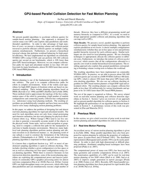
Abstract<br />
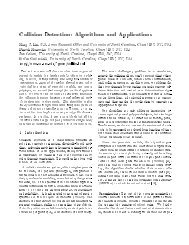
<strong>GPU</strong>-<strong>based</strong> <strong>Parallel</strong> <strong>Collision</strong> <strong>Detection</strong> <strong>for</strong> <strong>Fast</strong> <strong>Motion</strong> <strong>Planning</strong><br />
Jia Pan and Dinesh Manocha<br />
Dept. of Computer Science, University of North Carolina at Chapel Hill<br />
{panj,dm}@cs.unc.edu<br />
We present parallel algorithms to accelerate collision queries <strong>for</strong><br />
sample-<strong>based</strong> motion planning. Our approach is designed <strong>for</strong><br />
current many-core <strong>GPU</strong>s and exploits data-parallelism and multithreaded<br />
capabilities. In order to take advantage of high numbers<br />
of cores, we present a clustering scheme and collision-packet<br />
traversal to per<strong>for</strong>m efficient collision queries on multiple configurations<br />
simultaneously. Furthermore, we present a hierarchical<br />
traversal scheme that per<strong>for</strong>ms workload balancing <strong>for</strong> high parallel<br />
efficiency. We have implemented our algorithms on commodity<br />
NVIDIA <strong>GPU</strong>s using CUDA and can per<strong>for</strong>m 500, 000 collision<br />
queries per second on our benchmarks, which is 10X faster than<br />
prior <strong>GPU</strong>-<strong>based</strong> techniques. Moreover, we can compute collisionfree<br />
paths <strong>for</strong> rigid and articulated models in less than 100 milliseconds<br />
<strong>for</strong> many benchmarks, almost 50-100X faster than current<br />
CPU-<strong>based</strong> PRM planners.<br />
1 Introduction<br />
<strong>Motion</strong> planning is one of the fundamental problems in algorithmic<br />
robotics. The goal is to compute collision-free paths <strong>for</strong><br />
robots in complex environments. Some of the widely used algorithms<br />
<strong>for</strong> high-DOF (degree-of-freedom) robots are <strong>based</strong> on randomized<br />
sampling. These include planning algorithms <strong>based</strong> on<br />
PRMs [Kavraki et al. 1996] and RRTs [Kuffner and LaValle 2000].<br />
These methods tend to approximate the topology of the free configuration<br />
space of the robot by generating a high number of random<br />
configurations and connecting nearby collision-free configurations<br />
(i.e. milestones) using local planning methods. The resulting algorithms<br />
are probabilistically complete and have been successfully<br />
used to solve many challenging motion planning problems.<br />
In this paper, we address the problem of designing fast and almost<br />
real-time planning algorithms <strong>for</strong> rigid and articulated models. The<br />
need <strong>for</strong> such algorithms arises not only from virtual prototyping<br />
and character animation, but also task planning <strong>for</strong> physical robots.<br />
Current robots (e.g. Willow Garage’s PR2) tend to use live sensor<br />
data to generate a reasonably accurate model of the objects in<br />
the physical world. Some tasks, such as robot navigation or grasping,<br />
need to compute a collision-free path <strong>for</strong> the manipulator in<br />
real-time to handle dynamic environments. Moreover, many highlevel<br />
task planning algorithms per<strong>for</strong>m motion planning and subtask<br />
execution in an interleaved manner, i.e. the planning result of<br />
one subtask is used to construct the <strong>for</strong>mulation of the following<br />
subtasks [Talamadupula et al. 2009]. A fast and almost real-time<br />
planning algorithm is important <strong>for</strong> these applications.<br />
It is known that a significant fraction (e.g. 90% or more) of randomized<br />
sampling algorithms is spent in collision checking. This<br />
includes checking whether a given configuration is in free-space or<br />
not as well as connecting two free-space configurations using a local<br />
planning algorithm. While there is extensive literature on fast<br />
intersection detection algorithms, some of the recent planning algorithms<br />
are exploiting the computational power and massive parallelism<br />
of commodity <strong>GPU</strong>s (graphics processing units) <strong>for</strong> almost<br />
real-time computation [Pan et al. 2010b; Pan et al. 2010a]. Current<br />
<strong>GPU</strong>s are high-throughput many-core processors, which offer high<br />
data-parallelism and can simultaneously execute a high number of<br />
threads. However, they have a different programming model and<br />
memory hierarchy as compared to CPUs. As a result, we need to<br />
design appropriate parallel collision and planning algorithms that<br />
can map well to <strong>GPU</strong>s.<br />
Main Results: We present a novel, parallel algorithm to per<strong>for</strong>m<br />
collision queries <strong>for</strong> sample-<strong>based</strong> motion planning. Our approach<br />
exploits parallelism at two levels: it checks multiple configurations<br />
simultaneously (whether they are in free space or not) and per<strong>for</strong>ms<br />
parallel hierarchy traversal <strong>for</strong> each collision query. Similar techniques<br />
are also used <strong>for</strong> local planning queries. We use clustering<br />
techniques to appropriately allocate the collision queries to different<br />
cores, Furthermore, we introduce the notion of collision-packet<br />
traversal, which ensures that all the configurations allocated to a<br />
specific core result in similar hierarchical traversal patterns. The resulting<br />
approach also exploits fine-grained parallelism corresponding<br />
to bounding volume overlap tests to balance the workload.<br />
The resulting algorithms have been implemented on commodity<br />
NVIDIA <strong>GPU</strong>s. In practice, we are able to process about 500, 000<br />
collision queries per second on a $400 NVIDIA GeForce 480 desktop<br />
<strong>GPU</strong>, which is almost 10X faster than prior <strong>GPU</strong>-<strong>based</strong> collision<br />
checking algorithms. We also use our collision checking algorithm<br />
<strong>for</strong> <strong>GPU</strong>-<strong>based</strong> motion planners of high-DOF rigid and articulated<br />
robots. The resulting planner can compute collision-free<br />
paths in less than 100 milliseconds <strong>for</strong> various benchmarks and appears<br />
to be 50-100X faster than CPU-<strong>based</strong> PRM planners.<br />
The rest of the paper is organized as follows. We survey related<br />
work on real-time motion planning and collision detection algorithms<br />
in Section 2. Section 3 gives an overview of our approach<br />
and we present parallel algorithm <strong>for</strong> collision queries in Section 4.<br />
We highlight the per<strong>for</strong>mance of our algorithm on different benchmarks<br />
in Section 5. A preliminary version of this work was presented<br />
in [Pan and Manocha 2011].<br />
2 Previous Work<br />
In this section, we give a brief overview of prior work in real-time<br />
motion planning and parallel algorithms <strong>for</strong> collision detection.<br />
2.1 Real-time <strong>Motion</strong> <strong>Planning</strong><br />
An excellent survey of various motion planning algorithms is given<br />
in [LaValle 2006]. Many parallel algorithms have also been proposed<br />
<strong>for</strong> motion planning by utilizing the properties of configuration<br />
spaces [Lozano-Perez and O’Donnell 1991]. The distributed<br />
representation [Barraquand and Latombe 1991] can be easily parallelized.<br />
In order to deal with high dimensional or difficult planning<br />
problems, distributed sampling-<strong>based</strong> techniques have been<br />
proposed [Plaku et al. 2007].<br />
The computational power of many-core <strong>GPU</strong>s has been used <strong>for</strong><br />
many geometric and scientific computations [Owens et al. 2007].<br />
The rasterization capabilities of a <strong>GPU</strong> can be used <strong>for</strong> real-time<br />
motion planning of low DOF robots [Hoff et al. 2000; Sud et al.<br />
2007] or improve sample generation in narrow passages [Pisula<br />
et al. 2000; Foskey et al. 2001]. Recently, <strong>GPU</strong>-<strong>based</strong> parallel motion<br />
planning algorithms have been proposed <strong>for</strong> rigid models [Pan<br />
et al. 2010b; Pan et al. 2010a].
2.2 <strong>Parallel</strong> <strong>Collision</strong> Queries<br />
Some of the widely used algorithms <strong>for</strong> collision checking are<br />
<strong>based</strong> on bounding volume hierarchies (BVH), such as k-DOP<br />
trees, OBB trees, AABB trees, etc [Lin and Manocha 2004]. Recent<br />
developments include parallel hierarchical computations on multicore<br />
CPUs [Kim et al. 2009; Tang et al. 2010] and <strong>GPU</strong>s [Lauterbach<br />
et al. 2010]. CPU-<strong>based</strong> approaches tend to rely on finegrained<br />
communication between processors, which is not suited <strong>for</strong><br />
current <strong>GPU</strong>-like architectures. On the other hand, <strong>GPU</strong>-<strong>based</strong> algorithms<br />
[Lauterbach et al. 2010] use work queues to parallelize<br />
the computation on multiple cores. All of these approaches are primarily<br />
designed to parallelize a single collision query.<br />
The capability to efficiently per<strong>for</strong>m high numbers of collision<br />
queries is essential in motion planning algorithms, e.g. multiple<br />
collision queries in milestone computation and local planning.<br />
Some of the prior algorithms per<strong>for</strong>m parallel queries in a simple<br />
manner: each thread handles a single collision query in an independent<br />
manner [Pan et al. 2010b; Pan et al. 2010a; Amato and Dale<br />
1999; Akinc et al. 2005]. Since current multi-core CPUs have the<br />
capability to per<strong>for</strong>m multiple-instruction multiple-data (MIMD)<br />
computations, these simple strategies can work well on CPUs. On<br />
the other hand, current <strong>GPU</strong>s offer high data parallelism and the<br />
ability to execute a high number of threads in parallel to overcome<br />
the high memory latency. As a result, we need new parallel collision<br />
detection algorithms to fully exploit their capabilities.<br />
3 Overview<br />
In this section, we first provide some background on current <strong>GPU</strong><br />
architectures. Next, we address some issues in designing efficient<br />
parallel algorithms to per<strong>for</strong>m collision queries.<br />
3.1 <strong>GPU</strong> Architectures<br />
In recent years, the focus in processor architectures has shifted<br />
from increasing clock rate to increasing parallelism. Commodity<br />
<strong>GPU</strong>s such as NVIDIA Fermi 1 have theoretical peak per<strong>for</strong>mance<br />
of Tera-FLOP/s <strong>for</strong> single precision computations and hundreds of<br />
Giga-FLOP/s <strong>for</strong> double precision computations. This peak per<strong>for</strong>mance<br />
is significantly higher as compared to current multi-core<br />
CPUs, thus outpacing CPU architectures [Lindholm et al. 2008] at<br />
relatively modest cost of $400 to $500. However, <strong>GPU</strong>s have different<br />
architectural characteristics and memory hierarchy, that impose<br />
some constraints in terms of designing appropriate algorithms.<br />
First, <strong>GPU</strong>s usually have a high number of independent cores (e.g.<br />
the newest generation GTX 480 has 15 cores and each core has<br />
32 streaming processors resulting in total of 480 processors while<br />
GTX 280 has 240 processors). Each of the individual cores is a vector<br />
processor capable of per<strong>for</strong>ming the same operation on several<br />
elements simultaneously (e.g. 32 elements <strong>for</strong> current <strong>GPU</strong>s). Secondly,<br />
the memory hierarchy on <strong>GPU</strong>s is quite different from that<br />
of CPUs and cache sizes on the <strong>GPU</strong>s are considerably smaller.<br />
Moreover, each <strong>GPU</strong> core can handle several separate tasks in parallel<br />
and switch between different tasks in the hardware when one<br />
of them is waiting <strong>for</strong> a memory operation to complete. This hardware<br />
multithreading approach is thus designed to hide the memory<br />
access latency. Thirdly, all <strong>GPU</strong> threads are logically grouped<br />
in blocks with a per-block high-speed shared memory, which provides<br />
a weak synchronization capability between the <strong>GPU</strong> cores.<br />
Overall, shared memory is a limited resource on <strong>GPU</strong>s: increasing<br />
the shared memory distributed <strong>for</strong> each thread can limit the ex-<br />
1 http://www.nvidia.com/object/fermi_<br />
architecture.html<br />
tent of parallelism. Finally, multiple <strong>GPU</strong> threads are physically<br />
managed and scheduled in the single-instruction, multiple-thread<br />
(SIMT) way, i.e. threads are grouped into chunks and each chunk<br />
executes one common instruction at a time. In contrast to singleinstruction<br />
multiple-data (SIMD) schemes, the SIMT scheme allows<br />
each thread to have its own instruction address counter and<br />
register state, and there<strong>for</strong>e, freedom to branch and execute independently.<br />
However, the <strong>GPU</strong>’s per<strong>for</strong>mance can reduce significantly<br />
when threads in the same chunk diverge considerably, because<br />
these diverging portions are executed in a serial manner <strong>for</strong><br />
all the branches. As a result, threads with coherent branching decisions<br />
(e.g. threads traversing the same paths in the BVH) are<br />
preferred on <strong>GPU</strong>s in order to obtain higher per<strong>for</strong>mance [Gunther<br />
et al. 2007]. All of these characteristics imply that – unlike CPUs<br />
– achieving high per<strong>for</strong>mance in current <strong>GPU</strong>s depends on several<br />
factors:<br />
1. Generating a sufficient number of parallel tasks so that all the<br />
cores are highly utilized.<br />
2. Developing parallel algorithms such that the total number of<br />
threads is even higher than the number of tasks, so that each<br />
core has enough work to per<strong>for</strong>m while waiting <strong>for</strong> data from<br />
relatively slow memory accesses.<br />
3. Assigning appropriate size <strong>for</strong> shared memory to accelerate<br />
memory accesses and not reduce the level of parallelism.<br />
4. Per<strong>for</strong>ming coherent or similar branching decisions <strong>for</strong> each<br />
parallel thread within a given chunk.<br />
These requirements impose constraints in terms of designing appropriate<br />
collision query algorithms.<br />
3.2 Notation and Terminology<br />
We define some terms and highlight the symbols used in the rest of<br />
the paper.<br />
chunk The minimum number of threads that <strong>GPU</strong>s manage,<br />
schedule and execute in parallel, which is also called warp<br />
in the <strong>GPU</strong> computing literature. The size of chunk (chunksize<br />
or warp-size) is 32 on current NVIDIA <strong>GPU</strong>s (e.g. GTX<br />
280 and 480).<br />
block The logical collection of <strong>GPU</strong> threads that can be executed<br />
on the same <strong>GPU</strong> core. These threads synchronize by using<br />
barriers and communicate via a small high-speed low-latency<br />
shared memory.<br />
BVHa The bounding volume hierarchy (BVH) tree <strong>for</strong> model a.<br />
It is a binary tree with L levels, whose nodes are ordered<br />
in the breadth-first order starting from the root node. The ith<br />
BVH node is denoted as BVHa[i] and its children nodes<br />
are BVHa[2i] and BVHa[2i + 1] with 1 ≤ i ≤ 2 L−1 − 1.<br />
The nodes at the l-th level of a BVH tree are represented as<br />
BVHa[k], 2 l ≤ k ≤ 2 l+1 − 1 with 0 ≤ l < L. The inner<br />
nodes are also called bounding volumes (BV) and the leaf<br />
nodes also have a link to the primitive triangles that are used<br />
to represent the model.<br />
BVTTa,b The bounding volume test tree (BVTT) represents recursive<br />
collision query traversal between two objects a, b. It<br />
is a 4-ary tree, whose nodes are ordered in the breadth-first<br />
order starting from the root node. The i-th BVTT node is<br />
denoted as BVTTa,b[i] ≡ (BVHa[m], BVHb[n]) or simply<br />
(m, n), which checks the BV or primitive overlap between<br />
nodes BVHa[m] and BVHb[n]. Here m = ⌊i− 4M +2<br />
⌋+2 3<br />
M ,<br />
n = {i − 4M +2<br />
} + 2 3<br />
M and M = ⌊log4 (3i − 2)⌋, where
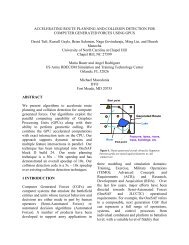
A<br />
B C<br />
<br />
D<br />
AD<br />
E F BE CE BE CF<br />
(a) Two BVH trees (b) BVTT tree<br />
Figure 1: BVH and BVTT: (a) shows two BVH trees and (b) shows<br />
the BVTT tree <strong>for</strong> the collision checking between the two BVH trees.<br />
{x} = x − ⌊x⌋. BVTT node (m, n)’s children are (2m, 2n),<br />
(2m, 2n + 1), (2m + 1, 2n), (2m + 1, 2n + 1).<br />
q A configuration of the robot, which is randomly sampled within<br />
the configuration space C-Space. q is associated with the<br />
trans<strong>for</strong>mation Tq. The BVH of a model a after applying<br />
such a trans<strong>for</strong>mation is given as BVHa(q).<br />
The relationship between BVH trees and BVTT is also shown in<br />
Figure 1. Notice that given the BVHs of two geometric models,<br />
the BVTT is completely determined using those BVHs and is independent<br />
of the actual configuration of each model. The model<br />
configurations only affect the actual traversal path of the BVTT.<br />
3.3 <strong>Collision</strong> Queries: Hierarchical Traversal<br />
<strong>Collision</strong> queries between the geometric models are usually accelerated<br />
with hierarchical techniques <strong>based</strong> on BVHs, which correspond<br />
to traversing the BVTT [Larsen et al. 2000]. The simplest<br />
parallel algorithms used to per<strong>for</strong>m multiple collision queries are<br />
<strong>based</strong> on each thread traversing the BVTT <strong>for</strong> one configuration<br />
and checking whether the given configuration is in free space or<br />
not. Such a simple parallel algorithm is highlighted in Algorithm 1.<br />
This strategy is easy to implement and has been used in previous<br />
parallel planning algorithms <strong>based</strong> on multi-core or multiple<br />
CPUs. But it may not result in high parallel efficiency on current<br />
<strong>GPU</strong>s due to the following reasons. First, each thread needs a local<br />
traversal stack <strong>for</strong> the BVTT. The stack size should be at least<br />
3(log 4 (Na) + log 4 (Nb))) to avoid stack overflow, where Na and<br />
Nb are the numbers of primitive triangles of BVHa and BVHb, respectively.<br />
The stack can be implemented using global memory<br />
or shared memory. Global memory access on the <strong>GPU</strong>s tends to<br />
be slow, which affects BVTT traversal. Shared memory access is<br />
much faster but it may be too small to hold the large stack <strong>for</strong> complex<br />
geometric models composed of thousands of polygons. Moreover,<br />
increasing the shared memory usage will limit the extent of<br />
parallelism. Second, different threads may traverse the BVTT tree<br />
with incoherent patterns: there are many branching decisions per<strong>for</strong>med<br />
during the traversal (e.g. loop, if, return in the pseudocode)<br />
and the traversal flow of the hierarchy in different threads<br />
diverges quickly. Finally, different threads can have varying workloads;<br />
some may be busy with the traversal while other threads may<br />
have finished the traversal early and are idle because there is no BV<br />
overlap or a primitive collision has already been detected. These<br />
factors can affect the per<strong>for</strong>mance of the parallel algorithm.<br />
The problems of low parallel efficiency in Algorithm 1 become<br />
more severe in complex or articulated models. For such models,<br />
there are longer traversal paths in the hierarchy and the difference<br />
between the length of these paths can be large <strong>for</strong> different configurations<br />
of a robot. As a result, differences in the workloads of<br />
different threads can be high. For articulated models, each thread<br />
checks the collision status of all the links and stops when a collision<br />
is detected <strong>for</strong> any link. There<strong>for</strong>e, more branching decisions<br />
are per<strong>for</strong>med within each thread and this can lead to more incoher-<br />
Algorithm 1 Simple parallel collision checking; such approaches<br />
are widely used on multi-core CPUs<br />
1: Input: N random configurations {qi} N i=1, BVHa <strong>for</strong> the robot<br />
and BVHb <strong>for</strong> the obstacles<br />
2: Output: return whether one configuration is in free space or not<br />
3: tid ← thread id of the current thread<br />
4: q ← qt id<br />
5: ⊳ traversal stack S[] is initialized with root nodes<br />
6: shared/global S[] ≡ local traversal stack<br />
7: S[] ←BVTT[1] ≡ (BVHa(q)[1],BVHb[1])<br />
8: ⊳ traverse BVTT <strong>for</strong> BVHa(q) and BVHb<br />
9: loop<br />
10: (x, y) ← pop(S).<br />
11: if overlap(BVHa(q)[x],BVHb[y]) then<br />
12: if !isLeaf(x) && !isLeaf(y) then<br />
13: S[] ← (2x, 2y), (2x, 2y + 1), (2x + 1, 2y), (2x +<br />
1, 2y + 1)<br />
14: end if<br />
15: if isLeaf(x) && !isLeaf(y) then<br />
16: S[] ← (2x, 2y), (2x, 2y + 1)<br />
17: end if<br />
18: if !isLeaf(x) && isLeaf(y) then<br />
19: S[] ← (2x, 2y), (2x + 1, 2y)<br />
20: end if<br />
21: if isLeaf(x) && isLeaf(y)&&<br />
exactIntersect(BVHa(q)[x],BVHb[y]) then<br />
22: return collision<br />
23: end if<br />
24: end if<br />
25: end loop<br />
26: return collision-free<br />
ent traversal. Similar issues also arise during local planning when<br />
each thread determines whether two milestones can be joined by a<br />
collision-free path by checking <strong>for</strong> collisions along the trajectory<br />
connecting them.<br />
4 <strong>Parallel</strong> <strong>Collision</strong> <strong>Detection</strong> on <strong>GPU</strong>s<br />
In this section, we present two novel algorithms <strong>for</strong> efficient parallel<br />
collision checking on <strong>GPU</strong>s between rigid or articulated models.<br />
Our methods can be used to check whether a configuration lies<br />
in the free space or to per<strong>for</strong>m local planning computations. The<br />
first algorithm uses clustering techniques and fine-grained packettraversal<br />
to improve the coherence of BVTT traversal <strong>for</strong> different<br />
threads. The second algorithm uses queue-<strong>based</strong> techniques and<br />
lightweight workload balancing to achieve higher parallel per<strong>for</strong>mance<br />
on the <strong>GPU</strong>s. In practice, the first method can provide 30%-<br />
50% speed up. Moreover, it preserves the per-thread per-query<br />
structure of the naive parallel strategy. There<strong>for</strong>e, it is easy to implement<br />
and is suitable <strong>for</strong> cases where we need to per<strong>for</strong>m some<br />
additional computations (e.g. retraction <strong>for</strong> handling narrow passages<br />
[Zhang and Manocha 2008]). The second method can provide<br />
5-10X speed up, but is relatively more complex to implement.<br />
4.1 <strong>Parallel</strong> <strong>Collision</strong>-Packet Traversal<br />
Our goal is to ensure that all the threads in a block per<strong>for</strong>ming<br />
BVTT-<strong>based</strong> collision checking have similar workloads and coherent<br />
branching patterns. This approach is motivated by recent developments<br />
related to interactive ray-tracing on <strong>GPU</strong>s <strong>for</strong> visual<br />
rendering. Each collision query traverses the BVTT and per<strong>for</strong>ms<br />
node-node or primitive-primitive intersection tests. In contrast, raytracing<br />
algorithms traverse the BVH tree and per<strong>for</strong>m ray-node or
ay-primitive intersections. There<strong>for</strong>e, parallel ray-tracing algorithms<br />
on <strong>GPU</strong>s also need to avoid incoherent branches and varying<br />
workloads to achieve higher per<strong>for</strong>mance.<br />
In real-time ray tracing, one approach to handle the varying workloads<br />
and incoherent branches is the use of ray-packets [Gunther<br />
et al. 2007; Aila and Laine 2009]. In ray-tracing terminology,<br />
packet traversal implies that a group of rays follow exactly the<br />
same traversal path in the hierarchy. This is achieved by sharing the<br />
traversal stack (similar to the BVTT traversal stack in Algorithm 1)<br />
among the rays in the same warp-sized packet (i.e. threads that fit<br />
in one chunk on the <strong>GPU</strong>), instead of each thread using an independent<br />
stack <strong>for</strong> a single ray. This implies that some additional nodes<br />
in the hierarchy may be visited during ray intersection tests, even<br />
though there are no intersections between the rays and those nodes.<br />
But the resulting traversal is coherent <strong>for</strong> different rays, because<br />
each node is fetched only once per packet. In order to reduce the<br />
number of computations (i.e. unnecessary node intersection tests),<br />
all the rays in one packet should be similar to one another, i.e. have<br />
similar traversal paths with few differing branches. For ray tracing,<br />
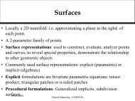
the packet construction is simple: as shown in Figure 2, rays<br />
passing through the same pixel on the image space make a natural<br />
packet. We extend this idea to parallel collision checking and refer<br />
to our algorithm as multiple configuration-packet method.<br />
Camera<br />
Ray Packet 2<br />
Image Space<br />
pixel<br />
Ray Packet 1<br />
Figure 2: Ray packets <strong>for</strong> faster ray tracing. Nearby rays constitute<br />
a ray packet and this spatial coherence is exploited <strong>for</strong> fast<br />
intersection tests.<br />
The first challenge is to cluster similar collision queries or the configurations<br />
into groups, because unlike ray tracing, there are no natural<br />
packet construction rules <strong>for</strong> collision queries. In some cases,<br />
the sampling scheme (e.g. the adaptive sampling <strong>for</strong> lazy PRM)<br />
can provide natural group partitions. However, in most cases we<br />
need suitable algorithms to compute these clusters. Clustering algorithms<br />
are natural choices <strong>for</strong> such a task, which aims at partitioning<br />
a set X of N data items {xi} N i=1 into K groups {Ck} K k=1 such<br />
that the data items belonging to the same group are more “similar”<br />
than the data items in different groups. The clustering algorithm<br />
used to group the configurations needs to satisfy some additional<br />
constraints: |Ck| = chunk-size, 1 ≤ k ≤ K. That is, each cluster<br />
should fit in one chunk on <strong>GPU</strong>s, except <strong>for</strong> the last cluster and<br />
K = ⌈ N<br />
⌉. Using the <strong>for</strong>mulation of k-means, the clustering<br />
chunk-size<br />
problem can be <strong>for</strong>mally described as:<br />
Compute K = ⌈ N<br />
chunk-size ⌉ items {ck} K k=1 that minimizes<br />
N<br />
i=1 k=1<br />
K<br />
1xi∈Ck xi − ck, (1)<br />
with constraints |Ck| = chunk-size, 1 ≤ k ≤ K. To our knowledge,<br />
there are no clustering algorithms designed <strong>for</strong> this specific<br />
problem. One possible solution is to use clustering with balancing<br />
constraints [Banerjee and Ghosh 2006], which has additional<br />
constraints |Ck| ≥ m, 1 ≤ k ≤ K, where m ≤ N<br />
K .<br />
Figure 3: Multiple configuration packet <strong>for</strong> parallel collision detection.<br />
Green points are random configuration samples in C-space.<br />
Grey areas are C-obstacles. Configurations adjacent in C-space are<br />
clustered into configuration packets (red circles). Some packets are<br />
completely in free space; some packets are completely within Cobstacles;<br />
some packets are near boundaries of C-obstacles. Configurations<br />
in the same packet have similar BVTT traversal paths<br />
and are mapped to the same warp on a <strong>GPU</strong>.<br />
Instead of solving Equation (1) exactly, we use a simpler clustering<br />
scheme to compute an approximate solution. First, we use k-means<br />
algorithm to cluster the N queries into C clusters, which can be<br />
implemented efficiently on <strong>GPU</strong>s [Che et al. 2008]. Next, <strong>for</strong> k-th<br />
Sk cluster of size Sk, we divide it into ⌈ ⌉ sub-clusters, each of<br />
chunk-size<br />
which corresponds to a configuration-packet. This simple method<br />
has some disadvantages. For example, the number of clusters is<br />
C Sk<br />
N<br />
⌈ ⌉ ≥ K = ⌈<br />
chunk-size chunk-size ⌉<br />
k=1<br />
and there<strong>for</strong>e Equation (1) may not result in an optimal solution.<br />
However, as shown later, even this simple method can improve the<br />
per<strong>for</strong>mance of parallel collision queries. The configuration clustering<br />
method is illustrated in Figure 3.<br />
Next we map each configuration-packet to a single chunk. Threads<br />
within one packet will traverse the BVTT synchronously, i.e. the<br />
algorithm works on one BVTT node (x, y) at a time and processes<br />
the whole packet against the node. If (x, y) is a leaf node, an exact<br />
intersection test is per<strong>for</strong>med <strong>for</strong> each thread. Otherwise, the algorithm<br />
loads its children nodes and tests the BVs <strong>for</strong> overlap to determine<br />
the remaining traversal order, i.e. to select one child (xm, ym)<br />
as the next BVTT node to be traversed <strong>for</strong> the entire packet. We select<br />
(xm, ym) in a greedy manner: it corresponds to the child node<br />
that is classified as overlapping by most threads in the packet. We<br />
also push other children into the packet’s traversal stack. In case<br />
no BV overlap is detected in all the threads or (x, y) is a leaf node,
(xm, ym) would be the top element in the packet’s traversal stack.<br />
The traversal step is repeated recursively, until the stack is empty.<br />
Compared to Algorithm 1, all the threads in one chunk share one<br />
traversal stack in shared memory, instead of using one stack <strong>for</strong><br />
each thread. There<strong>for</strong>e, the size of shared memory used is reduced<br />
by the chunk-size and results in higher parallel efficiency. The details<br />
of the traversal order decision rule is shown in Figure 4.<br />
The traversal order described above is a greedy heuristic that tries<br />
to minimize the traversal path of the entire packet. For one BVTT<br />
node (x, y), if the overlap is not detected in any of the threads, it<br />
implies that these threads will not traverse the sub-tree rooted at<br />
(x, y). Since all the threads in the packet are similar and traverse<br />
the BVTT in nearly identical order, this implies that other threads<br />
in the same packet might not traverse the sub-tree either. We define<br />
the probability that the sub-tree rooted at (x, y) will be traversed by<br />
one thread as<br />
px,y =<br />
number of overlap threads<br />
.<br />
packet-size<br />
For any traversal pattern P <strong>for</strong> BVTT, the probability that it is carried<br />
on by BVTT traversal will be<br />
pP = <br />
(x,y)∈P<br />
px,y.<br />
As a result, our new traversal strategy guarantees that the traversal<br />
pattern with higher traversal probability will have a shorter traversal<br />
length, and there<strong>for</strong>e minimizes the overall path <strong>for</strong> the packet.<br />
The decision about which child node is the candidate <strong>for</strong> next<br />
traversal step is computed using sum reduction [Harris 2009],<br />
which can compute the sum of n items in parallel with O(log(n))<br />
complexity. Each thread writes a 1 in its own location in the shared<br />
memory if it detects overlap in one child and 0 otherwise. The<br />
sum of the memory locations is computed in 5 steps <strong>for</strong> a size<br />
32 chunk. The packet chooses the child node with the maximum<br />
sum. The complete algorithm <strong>for</strong> configuration-packet computation<br />
is described in Algorithm 2.<br />
4.2 <strong>Parallel</strong> <strong>Collision</strong> Query with Workload Balancing<br />
Both Algorithm 1 and Algorithm 2 use the per-thread per-query<br />
strategy, which is relatively easy to implement. However, when the<br />
idle threads wait <strong>for</strong> busy threads or when the execution path of<br />
threads diverges, the parallel efficiency on the <strong>GPU</strong>s reduces. Algorithm<br />
2 can alleviate this problem in some cases, but it still distributes<br />
the tasks among the separate <strong>GPU</strong> cores and cannot make<br />
full use of the <strong>GPU</strong>’s computational power.<br />
In this section, we present the parallel collision query algorithm<br />
<strong>based</strong> on workload balancing which further improves the per<strong>for</strong>mance.<br />
In this algorithm, the task of each thread is no longer one<br />
complete collision query or continuous collision query (<strong>for</strong> local<br />
planning). Instead, each thread only per<strong>for</strong>ms BV overlap tests. In<br />
other words, the unit task <strong>for</strong> each thread is distributed in a more<br />
fine-grained manner. Basically, we <strong>for</strong>mulate the problem of per<strong>for</strong>ming<br />
multiple collision queries as a pool of BV overlap tests<br />
which can be per<strong>for</strong>med in parallel. It is easier to distribute these<br />
fine-grained tasks in a uni<strong>for</strong>m manner onto all the <strong>GPU</strong> cores,<br />
thereby balancing the load among them, than to distribute the collision<br />
query tasks.<br />
All the tasks are stored in large work queues in <strong>GPU</strong>’s main memory,<br />
which has a higher latency compared to the shared memory.<br />
When computing a single collision query [Lauterbach et al. 2010],<br />
the tasks are in the <strong>for</strong>m of BVTT nodes (x, y). Each thread will<br />
Algorithm 2 Multiple Configuration-Packet Traversal<br />
1: Input: N random configurations {qi} N i=1, BVHa <strong>for</strong> the robot<br />
and BVHb <strong>for</strong> the obstacles<br />
2: tid ← thread id of current thread<br />
3: q ← qt id<br />
4: shared CN[]≡ shared memory <strong>for</strong> children node<br />
5: shared T S[]≡ local traversal stack<br />
6: shared SM[]≡ memory <strong>for</strong> sum reduction<br />
7: if overlap(BVHa(q)[1], BVHb[1]) is false <strong>for</strong> all threads in<br />
chunk then<br />
8: return<br />
9: end if<br />
10: (x, y) = (1, 1)<br />
11: loop<br />
12: if isLeaf(x) && isLeaf(y) then<br />
13: if exactIntersect(BVHa(q)[x],BVHb[y]) then<br />
14: update collision status of q<br />
15: end if<br />
16: if T S is empty then<br />
17: break<br />
18: end if<br />
19: (x, y) ← pop(T S)<br />
20: else<br />
21: ⊳ decide the next node to be traversed<br />
22: CN[] ← (x, y)’s children nodes<br />
23: <strong>for</strong> all (xc, yc) ∈ CN do<br />
24: ⊳ compute the number of threads that detect overlap<br />
at node (xc, yc)<br />
25: write overlap(BVHa(q)[xc],BVHb[yc]) (0 or 1) into<br />
SM[tid] accordingly<br />
26: compute local summation sc in parallel by all threads<br />
in chunk<br />
27: end <strong>for</strong><br />
28: if maxc sc > 0 then<br />
29: ⊳ select the node that is overlapped in the most threads<br />
30: (x, y) ← CN[argmax c sc] and push others into T S<br />
31: else<br />
32: ⊳ select the node from the top of stack<br />
33: if T S is empty then<br />
34: break<br />
35: end if<br />
36: (x, y) ← pop(T S)<br />
37: end if<br />
38: end if<br />
39: end loop<br />
fetch some tasks from one work queue into its local work queue on<br />
the shared memory and traverse the corresponding BVTT nodes.<br />
The children generated <strong>for</strong> each node are also pushed into the local<br />
queue as new tasks. This process is repeated <strong>for</strong> all the tasks<br />
remaining in the queue, until the number of threads with full or<br />
empty local work queues exceeds a given threshold (we use 50% in<br />
our implementation) and non-empty local queues are copied back<br />
to the work queues on main memory. Since each thread per<strong>for</strong>ms<br />
simple tasks with few branches, our algorithm can make full use of<br />
<strong>GPU</strong> cores if there is a sufficient number of tasks in all the work<br />
queues. However, during the BVTT traversal, the tasks are generated<br />
dynamically and thus different queues may have varying numbers<br />
of tasks and this can lead to an uneven workload among the<br />
<strong>GPU</strong> cores. We use a balancing algorithm that redistributes the<br />
tasks among work queues (Figure 5). Suppose the number of tasks<br />
in each work queue is<br />
ni, 1 ≤ i ≤ Q.
0<br />
0<br />
0<br />
①<br />
1<br />
1 0<br />
② ③<br />
0<br />
1<br />
④ ⑤<br />
1<br />
0<br />
0<br />
0<br />
0<br />
0<br />
0<br />
0<br />
0<br />
0<br />
1<br />
0 1<br />
0<br />
0<br />
0<br />
0<br />
1<br />
1<br />
0<br />
0<br />
0<br />
0<br />
0<br />
0<br />
1<br />
① ② ① ② ① ②<br />
⑭<br />
④<br />
⑫<br />
0 1<br />
0<br />
0<br />
0<br />
0<br />
0<br />
0<br />
1<br />
1<br />
0<br />
0<br />
0<br />
0<br />
1<br />
0 1<br />
③ ③ ④ ③ ④<br />
⑤ ⑤ ⑤ ⑥<br />
⑬ ⑪<br />
⑧<br />
⑨<br />
⑩ ⑦<br />
⑤<br />
①<br />
⑥ ③<br />
Figure 4: Synchronous BVTT traversal <strong>for</strong> packet configurations. The four trees in the first row are the BVTT trees <strong>for</strong> configurations in<br />
the same chunk. For convenience, we represent BVTT as binary tree instead of 4-ary tree. The 1 or 0 at each node represents whether the<br />
BV-overlap or exact intersection test executed at that node is in-collision or collision-free. The red edges are the edges visited by the BVTT<br />
traversal algorithm and the indices on these edges represent the traversal order. In this case, the four different configurations have traversal<br />
paths of length 5, 5, 5 and 6. The leaf nodes with red 1 are locations where collisions are detected and the traversal stop. The tree in<br />
the second row shows the synchronous BVTT traversal order determined by our heuristic rule, which needs to visit 10 edges to detect the<br />
collisions of all the four configurations.<br />
Whenever there exists i so that ni < Tl or ni > Tu, we execute<br />
our balancing algorithm among all the queues and the number of<br />
tasks in each queue becomes<br />
n ∗ Q i =<br />
k=1 nk<br />
, 1 ≤ i ≤ Q,<br />
Q<br />
where Tl and Tu are two thresholds (we use chunk-size <strong>for</strong> Tl and<br />
the W − chunk-size <strong>for</strong> Tu, where W is the maximum size of work<br />
queue).<br />
In order to handle N collision queries simultaneously, we use several<br />
strategies, which are highlighted and compared in Figure 6.<br />
First, we can repeat the single query algorithm [Lauterbach et al.<br />
2010] introduced above <strong>for</strong> each query. However, this has two main<br />
disadvantages. First, the <strong>GPU</strong> kernel has to be called N times from<br />
the CPU, which is expensive <strong>for</strong> large N (which can be ≫ 10000<br />
<strong>for</strong> sample-<strong>based</strong> motion planning). Secondly, <strong>for</strong> each query, work<br />
queues are initialized with only one item (i.e. the root node of the<br />
BVTT), there<strong>for</strong>e the <strong>GPU</strong>’s computational power cannot be fully<br />
exploited at the beginning of each query, as shown in the slow ascending<br />
part in Figure 6(a). Similarly, at the end of each query,<br />
most tasks have been finished and some of the <strong>GPU</strong> cores become<br />
idle, which corresponds to the slow descending part in Figure 6(a).<br />
As a result, we use the strategy shown in Figure 6(b): we divide the<br />
N queries into ⌈ N<br />
⌉ different sets each of size M with M ≤ N<br />
M<br />
and initialize the work queues with M different BVTT roots <strong>for</strong><br />
each iteration. Usually M cannot be N because we need to use<br />
t · M <strong>GPU</strong> global memory to store the trans<strong>for</strong>m in<strong>for</strong>mation <strong>for</strong><br />
the queries, where constant<br />
t ≤<br />
size of global memory<br />
M<br />
②<br />
④<br />
and we usually use M = 50. In this case, we only need to invoke<br />
the solution kernel ⌈ N<br />
⌉ times. The number of tasks available in<br />
M<br />
the work queues changes more smoothly over time, with fewer ascending<br />
and descending parts, which implies higher throughput of<br />
the <strong>GPU</strong>s. Moreover, the work queues are initialized with many<br />
more tasks, which results in high per<strong>for</strong>mance at the beginning of<br />
each iteration. In practice, as nodes from more than one BVTT of<br />
different queries co-exist in the same queue, we need to distinguish<br />
them by representing each BVTT node by (x, y, i) instead of (x, y),<br />
where i is the index of collision query. The details <strong>for</strong> this strategy<br />
are shown in Algorithm 3.<br />
We can further improve the efficiency by using the pump operation,<br />
as shown in Algorithm 4 and Figure 5. That is, instead of<br />
initializing the work queues after it is completely empty, we add<br />
M BVTT root nodes of unresolved collision queries into the work<br />
queues when the number of tasks in it decreases to a threshold (we<br />
use 10 · chunk-size). As a result, the few ascending and descending<br />
parts in Figure 6(b) can be further flattened as shown in Figure<br />
6(c). Pump operation can reduce the timing overload of interrupting<br />
traversal kernels or copying data between global memory<br />
and shared memory, and there<strong>for</strong>e improve the overall efficiency of<br />
collision computation.<br />
4.3 Analysis<br />
In this section, we analyze the algorithms described above using the<br />
parallel random access machine (PRAM) model, which is a popular<br />
tool to analyze the complexity of parallel algorithms [JáJá 1992].<br />
Of course, current <strong>GPU</strong> architectures have many properties that can<br />
not be described by PRAM model, such as SIMT, shared memory,<br />
etc. However, PRAM analysis can still provide some insight into<br />
<strong>GPU</strong> algorithm’s per<strong>for</strong>mance.<br />
0<br />
0<br />
0<br />
0<br />
0<br />
0<br />
0<br />
1<br />
1
Algorithm 3 Traversal with Workload Balancing: Task Kernel<br />
1: Input: abort signal signal, N random configurations {qi} N i=1,<br />
BVHa <strong>for</strong> the robot and BVHb <strong>for</strong> the obstacles<br />
2: shared W Q[] ≡ local work queue<br />
3: initialize W Q by tasks in global work queues<br />
4: ⊳ traverse on work queues instead of BVTTs<br />
5: loop<br />
6: (x, y, i) ← pop(W Q)<br />
7: if overlap(BVHa(qi)[x],BVHb[y]) then<br />
8: if isLeaf(x) && isLeaf(y) then<br />
9: if exactIntersect(BVHa(qi)[x],BVHb[y]) then<br />
10: update collision status of i-th query<br />
11: end if<br />
12: else<br />
13: W Q[] ← (x, y, i)’s children<br />
14: end if<br />
15: end if<br />
16: if W Q is full or empty then<br />
17: atomically increment signal, break<br />
18: end if<br />
19: end loop<br />
20: return if signal > 50%Q<br />
Algorithm 4 Traversal with Workload Balancing: Manage Kernel<br />
1: Input: Q global work queues<br />
2: copy local queues on shared memory back to Q global work<br />
queues on global memory<br />
3: compute the number of tasks in each work queue ni, 1 ≤ i ≤<br />
Q<br />
4: compute the number of tasks in all queues n = Q k=1 nk<br />
5: if n < Tpump then<br />
6: call pump kernel: add more tasks in global queue from unresolved<br />
collision queries<br />
7: else if ∃i, ni < Tl||ni > Tu then<br />
8: call balance kernel: rearrange the tasks so that each queue<br />
has n ∗ Q k=1<br />
i =<br />
nk tasks<br />
Q<br />
9: end if<br />
10: call task kernel again<br />
Suppose we are given n collision queries, which means that we<br />
need to traverse n BVTT of the same tree structure but with different<br />
geometry configurations. We denote the complexity of serial<br />
algorithm as TS(n), the complexity of naive parallel algorithm<br />
(Algorithm 1) as TN (n), the complexity of configuration-packet<br />
algorithm (Algorithm 2) as TP (n) and the complexity of workload<br />
balancing algorithm (Algorithm 4) as TB(n). Then we have the<br />
following result:<br />
Lemma 1 Θ(TS(n)) = TN (n) ≥ TP (n) ≥ TB(n).<br />
Remark In parallel computing, we say one parallel algorithm is<br />
work efficient, if its complexity T (n) is bounded both above and<br />
below asymptotically by S(n), the complexity of its serial version,<br />
i.e. T (n) = Θ(S(n)) [JáJá 1992]. In other words, Lemma 1 means<br />
that all the three parallel collision algorithms are work-efficient,<br />
but the workload balancing is the most efficient and configurationpacket<br />
algorithm is more efficient than the naive parallel scheme.<br />
Proof Let the complexity to traverse the i-th BVTT be W (i),<br />
1 ≤ i ≤ n. Then the complexity of a sequential CPU algorithm<br />
is TS(n) = n i=1 W (i). For <strong>GPU</strong>-<strong>based</strong> parallel algorithms, we<br />
assume that the <strong>GPU</strong> has p processors or cores. For convenience,<br />
we assume n = ap, a ∈ Z.<br />
Core 1<br />
Task 0<br />
Task i<br />
External<br />
Task<br />
Pools<br />
…<br />
pump kernel<br />
abort or<br />
continue<br />
Global<br />
Task Pools<br />
Global<br />
Task Pools<br />
……<br />
Task k<br />
Utilization<br />
Core k<br />
…<br />
Task k+i<br />
manage kernel<br />
balance kernel<br />
abort or<br />
continue<br />
……<br />
……<br />
……<br />
Task n<br />
Core n<br />
…<br />
Task n+i<br />
abort or<br />
continue<br />
full<br />
empty<br />
full<br />
empty<br />
Figure 5: Load balancing strategy <strong>for</strong> our parallel collision query<br />
algorithm. Each thread keeps its own local work queue in local<br />
memory. After processing a task, each thread is either able to<br />
run further or has an empty or full work queue and terminates.<br />
Once the number of <strong>GPU</strong> cores terminated exceeds a given threshold,<br />
the manage kernel is called and copies the local queues back<br />
onto global work queues. If no work queue has too many or too<br />
few tasks, the task kernel restarts. Otherwise, the balance kernel<br />
is called to balance the tasks among all the queues. If there are<br />
not sufficient tasks in the queues, more BVTT root nodes will be<br />
’pumped’ in by the pump kernel.<br />
For a naive parallel algorithm (Algorithm 1), each processor executes<br />
BVTT traversal independently and the overall per<strong>for</strong>mance is<br />
determined by the most time-consuming BVTT traversal. There<strong>for</strong>e,<br />
its complexity becomes<br />
a−1 p<br />
TN (n) = max W (kp + j).<br />
j=1<br />
k=0<br />
If we sort {W (i)} n i=1 in ascending order and denote W ∗ (i) as the<br />
i-th element in the new order, we have<br />
a−1 p<br />
max W (kp + j) ≥<br />
j=1<br />
k=0<br />
task kernel<br />
a<br />
W ∗ (kp). (2)<br />
k=1<br />
To prove it, we start from a = 2. In this case, the summation<br />
max p<br />
j=1 W (j) + maxpj=1<br />
W (p + j) achieves the minimum when<br />
min {W (p + 1), · · · , W (2p)} ≥ max {W (1), · · · , W (p)}. Otherwise,<br />
exchange the minimum value in {W (p + 1), · · · , W (2p)}<br />
and the maximum value in {W (1), · · · , W (p)} will increase the<br />
summation. For a > 2, using similarly technique, we can show<br />
that the minimum of a−1 k=0 maxpj=1<br />
W (kp + j) happens when<br />
min (j+1)p<br />
k=jp+1 {W (k)} ≥ maxjp (j−1)p+1 {W (k)}, 1 ≤ j ≤ a − 1.<br />
This is satisfied by the ascending sorted result W ∗ and the Inequality<br />
(2) is proved.<br />
Moreover, it is obvious that n i=1 W (i) ≥ TN (n) ≥<br />
Then we obtain<br />
TS(n) ≥ TN (n) ≥ max TS(n)<br />
p<br />
,<br />
a<br />
W ∗ (kp) ,<br />
k=1<br />
ni=1 W (i)<br />
p<br />
.
throughput<br />
throughput<br />
throughput<br />
(a)<br />
(b)<br />
(c)<br />
Figure 6: Different strategies <strong>for</strong> parallel collision query using<br />
work queues. (a) Naive way: repeat the single collision query<br />
algorithm one by one; (b) Work queues are initialized by some<br />
BVTT root nodes and we repeat the process until all queries are<br />
per<strong>for</strong>med. (c) is similar to (b) except that new BVTT root nodes<br />
are added to the work queues by the pump kernel, when there is not<br />
sufficient number of tasks in the queue.<br />
which implies TN (n) = Θ(TS(n)).<br />
According to the analysis in Section 4.1, we know that the expected<br />
complexity ˆ W (i) <strong>for</strong> i-th BVTT traversal in configuration-packet<br />
method (Algorithm 2) should be smaller than W (i) because of the<br />
near-optimal traversing order. Moreover, the clustering strategy is<br />
similar to ordering different BVTTs, so that the BVTTs with similar<br />
traversal paths are arranged closely to each other and thus the probability<br />
is higher that they would be distributed on the same <strong>GPU</strong><br />
core. In practice, we can not implement such an ordering exactly<br />
because the complexity of BVTT traversal is not known a priori.<br />
There<strong>for</strong>e the complexity of Algorithm 2 is<br />
TP (n) ≈<br />
a<br />
ˆW ∗ (kp),<br />
k=1<br />
with ˆ W ∗ ≤ W ∗ . As a result, we have TP (n) ≤ TN (n).<br />
The complexity <strong>for</strong> workload balancing method (Algorithm 4) can<br />
be given as:<br />
n i=1 W (i)<br />
TB(n) =<br />
+ B(n),<br />
p<br />
where the first item is the timing complexity <strong>for</strong> BVTT traversal and<br />
the second item B(n) is the timing complexity <strong>for</strong> balancing step.<br />
As B(n) > 0, the acceleration ratio of <strong>GPU</strong> with p-processors is<br />
less than p. We need to reduce the load of balancing step to improve<br />
the efficiency of Algorithm 4. If balancing step is implemented<br />
efficiently, i.e. if B(n) = o(TS(n)), we have TN (n) ≥ TP (n) ≥<br />
TB(n).<br />
5 Implementation and Results<br />
In this section, we present some details of the implementation and<br />
highlight the per<strong>for</strong>mance of our algorithm on different benchmarks.<br />
All the timings reported here were recorded on a machine<br />
using an Intel Core i7 3.2GHz CPU and 6GB memory. We implemented<br />
our collision and planning algorithms using CUDA on a<br />
NVIDIA GTX 480 <strong>GPU</strong> with 1GB of video memory.<br />
time<br />
time<br />
time<br />
Query phase<br />
Roadmap construction<br />
PRM algorithm <strong>GPU</strong> algorithm<br />
Sample generation<br />
s samples<br />
Milestone construction<br />
m milestones (m
piano large-piano helicopter humanoid PR2<br />
#robot-faces 6,540 34,880 3,612 27,749 31,384<br />
#obstace-faces 648 13,824 2,840 3,495 3,495<br />
DOF 6 6 6 38 12 (one arm)<br />
Table 1: Geometric complexity of our benchmarks. Large-piano is a piano model that has more vertices and faces and is obtained by<br />
subdividing the original piano model.<br />
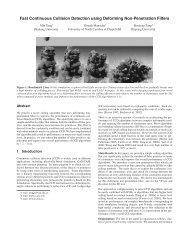
(a) piano (b) helicopter<br />
(c) humanoid (d) PR2<br />
Figure 8: Benchmarks used in our experiments.<br />
In order to compare the per<strong>for</strong>mance of different parallel collision<br />
detection algorithms, we use the benchmarks shown in Figure 8.<br />
The geometric complexity of these benchmarks is shown in Table<br />
1. For rigid body benchmarks, we generate 50, 000 random<br />
configurations and compute a collision-free path by using different<br />
variants of our parallel collision detection algorithm. For articulated<br />
model benchmark, we generate 100, 000 random configurations.<br />
For milestone computation, we directly use our collision detection<br />
algorithm. For local planning, we first need to unfold all the<br />
interpolated configurations: we denote the BVTT <strong>for</strong> the j-th interpolated<br />
query between the i-th local path as BVTT(i, j) and its<br />
node as (x, y, i, j). In order to avoid unnecessary computations, we<br />
first add BVTT root nodes with small j into the work queues, i.e.<br />
(1, 1, i, j) ≺ (1, 1, i ′ , j ′ ), ifj < j ′ . As a result, once a collision is<br />
computed at BVTT(i, j0), we need not traverse BVTT(i, j) when<br />
j > j0.<br />
For Algorithm 1 and Algorithm 2, we further test the per<strong>for</strong>mance<br />
<strong>for</strong> different traversal sizes (i.e. 32 and 128). Both algorithms give<br />
correct results when using a larger stack size (i.e. 128). For smaller<br />
stack sizes, the algorithms will stop once the stack is filled. Algorithm<br />
1 may report a collision when the stack overflows while<br />
Algorithm 2 returns a collision-free query. There<strong>for</strong>e, Algorithm 1<br />
may suffer from false positive errors while Algorithm 2 may suffer<br />
from false negative errors. We also compare the per<strong>for</strong>mance of Algorithm<br />
1 and Algorithm 2 when the clustering algorithm described<br />
in Section 4.1 is used and when it is not.<br />
The timing results are shown in Table 2 and Table 3. We observe:<br />
(1) Algorithm 1 and Algorithm 2 both work better when<br />
local traversal stack is smaller and pre-clustering technique is used.<br />
However <strong>for</strong> large models, traversal stack of size 32 may result in<br />
overflows and the collision results can be incorrect, which happens<br />
<strong>for</strong> the large-piano benchmarks in Table 2 and Table 3. Algorithm<br />
1’s per<strong>for</strong>mance is considerably reduced when the size of<br />
Figure 9: Our <strong>GPU</strong>-<strong>based</strong> motion planner can compute a<br />
collision-free path <strong>for</strong> PR2 in less than 1 second.<br />
traversal stack increases to 128. This is due to the fact that Algorithm<br />
2 uses per-packet stack, which is about 32 times smaller then<br />
using per-thread stack. Moreover, clustering and configurationpacket<br />
traversal can result in more than 50% speed-up. Moreover,<br />
the improvement in the per<strong>for</strong>mance of Algorithm 2 over Algorithm<br />
1 is more on complex models (e.g. large-piano). (2) Algorithm<br />
4 is usually the fastest one among all the variations of the<br />
three algorithms. It can result in more than 5-10X speedup over<br />
other methods.<br />
As observed in [Pan et al. 2010b; Pan et al. 2010a], the per<strong>for</strong>mance<br />
of the planner in these benchmarks is dominated by milestone computation<br />
and local planning. Based on the novel collision detection<br />
algorithm, the per<strong>for</strong>mance of PRM and lazy PRM planners can be<br />
improved by at least 40%-45%.<br />
In Figure 10, we also show how the pump kernel increases the<br />
<strong>GPU</strong> throughput (i.e. the number of tasks available in work queues<br />
<strong>for</strong> <strong>GPU</strong> cores to fetch) in the workload balancing <strong>based</strong> Algorithm<br />
4. The maximum throughput (i.e. the maximum number<br />
of BV overlap tests per<strong>for</strong>med by <strong>GPU</strong> kernels) increases from<br />
8 × 10 4 to nearly 10 5 and the minimum throughput increases from<br />
0 to 2.5 × 10 4 . For piano and helicopter models, we can compute<br />
a collision-free path from the initial to the goal configuration<br />
in 879ms and 778ms, respectively, using PRM or 72.79ms or<br />
72.68ms, respectively, using lazy PRM.<br />
5.3 Articulated Models<br />
Our parallel algorithms can be directly applied to articulated models.<br />
In this case, checking <strong>for</strong> self-collisions among various links<br />
of a robot adds to the overall complexity. We use a model of the<br />
PR2 robot as an articulated benchmark. The PR2 robot model has<br />
65 links and 75 DOFs. We only allow one arm (i.e. 12 DOFs)<br />
to be active in terms of motion. A naive approach would involve<br />
exhaustive self-collision checking, and reduces to checking<br />
65 × (65 − 1)/2 = 2, 080 self-collisions among the links <strong>for</strong> each<br />
collision query. As shown in Table 4, <strong>GPU</strong>-<strong>based</strong> planner takes<br />
more than 10 seconds <strong>for</strong> the PR2 benchmark when per<strong>for</strong>ming ex-
Algorithm 1 Algorithm 2 Algorithm 4<br />
32, no-C 32, C 128, no-C 128, C 32, no-C 32, C 128, no-C 128, C traversal balancing<br />
piano 117 113 239 224 177 131 168 130 68 3.69<br />
large-piano 409 387 738 710 613 535 617 529 155 15.1<br />
helicopter 158 151 286 272 224 166 226 163 56 2.3<br />
humanoid 2,392 2,322 2,379 2,316 2,068 1,877 2,073 1,823 337 106<br />
Table 2: Comparison of different algorithms in milestone computation (timing in milliseconds). 32 and 128 are the different sizes used <strong>for</strong><br />
the traversal stack; C and no-C means using pre-clustering and not using pre-clustering, respectively; timing of Algorithm 4 includes two<br />
parts: traversal part and balancing part.<br />
Algorithm 1 Algorithm 2 Algorithm 4<br />
32, no-C 32, C 128, no-C 128, C 32, no-C 32, C 128, no-C 128, C traversal balancing<br />
piano 1,203 1,148 2,213 2,076 1,018 822 1,520 1,344 1,054 34<br />
large-piano 4,126 3,823 8,288 7,587 5,162 4,017 7,513 6,091 1,139 66<br />
helicopter 4,528 4,388 7,646 7,413 3,941 3,339 5,219 4,645 913 41<br />
humanoid 5,726 5,319 9,273 8,650 4,839 4,788 9,012 8,837 6,082 1,964<br />
Table 3: Comparison of different algorithms in local planning (timing in milliseconds). 32 and 128 are the different sizes used <strong>for</strong> the<br />
traversal stack; C and no-C means using pre-clustering and not using pre-clustering, respectively; timing of Algorithm 4 includes two parts:<br />
traversal part and balancing part.<br />
haustive self-collision, though it is still much faster than the CPU<strong>based</strong><br />
implementation.<br />
However, exhaustive self-collision checking is usually not necessary<br />
<strong>for</strong> physical robots, because the joint limits can filter out many<br />
of the self-collisions. The common method is to manually set some<br />
link pairs that need to be checked <strong>for</strong> self-collisions. This strategy<br />
can greatly reduce the number of pairwise checks. As shown in<br />
Table 4, we can compute a collision-free path <strong>for</strong> the PR2 model<br />
in less than 1 seconds, which can be further reduced to 300ms if<br />
the number of samples is reduced to 500. The collision-free path<br />
calculated by our planner is shown in Figure 9.<br />
6 Conclusion and Future Work<br />
In this paper, we introduce two novel parallel collision query algorithms<br />
<strong>for</strong> real-time motion planning on <strong>GPU</strong>s. The first algorithm<br />
is <strong>based</strong> on configuration-packet tracing, is easy to implement, and<br />
can improve the parallel per<strong>for</strong>mance by per<strong>for</strong>ming more coherent<br />
traversals and reducing the memory consumed by traversal stacks.<br />
It can provide more than 50% speed-up as compared to simple parallel<br />
methods. The second algorithm is <strong>based</strong> on workload balancing,<br />
and decomposes parallel collision queries into fine-grained<br />
tasks corresponding to BVTT node operations. The algorithm uses<br />
a light-weight task-balancing strategy to guarantee that all <strong>GPU</strong><br />
cores are fully utilized and achieves close to peak per<strong>for</strong>mance on<br />
<strong>GPU</strong>s. In practice, we observe 5-10X speed-up. The new collision<br />
algorithms can improve the per<strong>for</strong>mance of <strong>GPU</strong>-<strong>based</strong> PRM<br />
planners by almost 50%.<br />
There are many avenues <strong>for</strong> future work. We are interested in using<br />
more advanced sampling schemes with the <strong>GPU</strong>-<strong>based</strong> planner<br />
to further improve its per<strong>for</strong>mance and deal with narrow passages.<br />
Furthermore, we would like to modify the planner to generate<br />
smooth paths and integrate our planner with physical robots<br />
(e.g. PR2). We would also like to take into account kinematic and<br />
dynamic constraints.<br />
Acknowledgements This work was supported in part by ARO<br />
Contract W911NF-04-1-0088, NSF awards 0636208, 0917040 and<br />
0904990, DARPA/RDECOM Contract WR91CRB-08-C-0137, and<br />
Willow Garage.<br />
References<br />
AILA, T., AND LAINE, S. 2009. Understanding the efficiency<br />
of ray traversal on <strong>GPU</strong>s. In Proceedings of High Per<strong>for</strong>mance<br />
Graphics, 145–149.<br />
AKINC, M., BEKRIS, K. E., CHEN, B. Y., LADD, A. M., PLAKU,<br />
E., AND KAVRAKI, L. E. 2005. Probabilistic roadmaps of trees<br />
<strong>for</strong> parallel computation of multiple query roadmaps. In Robotics<br />
Research, vol. 15 of Springer Tracts in Advanced Robotics.<br />
Springer, 80–89.<br />
AMATO, N., AND DALE, L. 1999. Probabilistic roadmap methods<br />
are embarrassingly parallel. In International Conference on<br />
Robotics and Automation, 688 – 694.<br />
BANERJEE, A., AND GHOSH, J. 2006. Scalable clustering algorithms<br />
with balancing constraints. Data Mining and Knowledge<br />
Discovery 13, 3, 365–395.<br />
BARRAQUAND, J., AND LATOMBE, J.-C. 1991. Robot motion<br />
planning: A distributed representation approach. International<br />
Journal of Robotics Research 10, 6.<br />
CHE, S., BOYER, M., MENG, J., TARJAN, D., SHEAFFER, J. W.,<br />
AND SKADRON, K. 2008. A per<strong>for</strong>mance study of generalpurpose<br />
applications on graphics processors using cuda. Journal<br />
of <strong>Parallel</strong> and Distributed Computing 68, 10, 1370–1380.<br />
FOSKEY, M., GARBER, M., LIN, M., AND MANOCHA, D. 2001.<br />
A voronoi-<strong>based</strong> hybrid planner. In Proceedings of IEEE International<br />
Conference on Intelligent Robots and Systems, 55 – 60.<br />
GUNTHER, J., POPOV, S., SEIDEL, H.-P., AND SLUSALLEK, P.<br />
2007. Realtime ray tracing on <strong>GPU</strong> with BVH-<strong>based</strong> packet<br />
traversal. In Proceedings of IEEE Symposium on Interactive Ray<br />
Tracing, 113–118.<br />
HARRIS, M., 2009. Optimizing parallel reduction in CUDA.<br />
NVIDIA Developer Technology.<br />
HOFF, K., CULVER, T., KEYSER, J., LIN, M., AND MANOCHA,<br />
D. 2000. Interactive motion planning using hardware accelerated<br />
computation of generalized voronoi diagrams. In Proceed-
milestone computation local planning<br />
exhaustive self-collision (CPU) 15,952 643,194<br />
exhaustive self-collision (<strong>GPU</strong>) 652 13,513<br />
manual self-collision (<strong>GPU</strong>) 391 392<br />
Table 4: <strong>Collision</strong> timing on PR2 benchmark (timing in milliseconds). We use 1, 000 samples, 20-nearest neighbor and discrete local<br />
planning with 20 interpolations. Manually self-collision setting can greatly improve the per<strong>for</strong>mance of <strong>GPU</strong> planner.<br />
<strong>GPU</strong> throughput<br />
<strong>GPU</strong> throughput<br />
x 104<br />
8<br />
7<br />
6<br />
5<br />
4<br />
3<br />
2<br />
1<br />
0<br />
0<br />
x 104<br />
10<br />
0.02 0.04 0.06<br />
timing<br />
0.08 0.1 0.12<br />
9<br />
8<br />
7<br />
6<br />
5<br />
4<br />
3<br />
2<br />
1<br />
0<br />
0 0.02 0.04 0.06<br />
timing<br />
0.08 0.1 0.12<br />
Figure 10: <strong>GPU</strong> throughput improvement caused by pump kernel.<br />
Left figure shows the throughput without using the pump kernel and<br />
right figure shows the throughput using the pump kernel.<br />
ings of IEEE International Conference on Robotics and Automation,<br />
2931 – 2937.<br />
JÁJÁ, J. 1992. An introduction to parallel algorithms. Addison<br />
Wesley Longman Publishing Co., Inc.<br />
KAVRAKI, L., SVESTKA, P., LATOMBE, J. C., AND OVER-<br />
MARS, M. 1996. Probabilistic roadmaps <strong>for</strong> path planning in<br />
high-dimensional configuration spaces. IEEE Transactions on<br />
Robotics and Automation 12, 4, 566–580.<br />
KIM, D., HEO, J.-P., HUH, J., KIM, J., AND YOON, S.-E. 2009.<br />
HPCCD: Hybrid parallel continuous collision detection using<br />
cpus and gpus. Computer Graphics Forum 28, 7, 1791–1800.<br />
KUFFNER, J., AND LAVALLE, S. 2000. RRT-connect: An efficient<br />
approach to single-query path planning. In Proceedings<br />
of IEEE International Conference on Robotics and Automation,<br />
995 – 1001.<br />
LARSEN, E., GOTTSCHALK, S., LIN, M., AND MANOCHA, D.<br />
2000. Distance queries with rectangular swept sphere volumes.<br />
In Proceedings of IEEE International Conference on Robotics<br />
and Automation, 3719–3726.<br />
LAUTERBACH, C., GARLAND, M., SENGUPTA, S., LUEBKE, D.,<br />
AND MANOCHA, D. 2009. <strong>Fast</strong> BVH construction on <strong>GPU</strong>s.<br />
Computer Graphics Forum 28, 2, 375–384.<br />
LAUTERBACH, C., MO, Q., AND MANOCHA, D. 2010. gProximity:<br />
Hierarchical <strong>GPU</strong>-<strong>based</strong> operations <strong>for</strong> collision and distance<br />
queries. Computer Graphics Forum 29, 2, 419–428.<br />
LAVALLE, S. M. 2006. <strong>Planning</strong> Algorithms. Cambridge University<br />
Press.<br />
LIN, M., AND MANOCHA, D. 2004. <strong>Collision</strong> and proximity<br />
queries. In Handbook of Discrete and Computational Geometry.<br />
CRC Press, Inc., 787–808.<br />
LINDHOLM, E., NICKOLLS, J., OBERMAN, S., AND MONTRYM,<br />
J. 2008. NVIDIA Tesla: A unified graphics and computing<br />
architecture. IEEE Micro 28, 2, 39–55.<br />
LOZANO-PEREZ, T., AND O’DONNELL, P. 1991. <strong>Parallel</strong> robot<br />
motion planning. In Proceedings of IEEE International Conference<br />
on Robotics and Automation, 1000–1007.<br />
OWENS, J. D., LUEBKE, D., GOVINDARAJU, N., HARRIS, M.,<br />
KRÜGER, J., LEFOHN, A. E., AND PURCELL, T. 2007. A<br />
survey of general-purpose computation on graphics hardware.<br />
Computer Graphics Forum 26, 1, 80–113.<br />
PAN, J., AND MANOCHA, D. 2011. <strong>GPU</strong>-<strong>based</strong> parallel collision<br />
detection <strong>for</strong> real-time motion planning. In Algorithmic Foundations<br />
of Robotics IX, vol. 68 of Springer Tracts in Advanced<br />
Robotics. Springer, 211–228.<br />
PAN, J., LAUTERBACH, C., AND MANOCHA, D. 2010. Efficient<br />
nearest-neighbor computation <strong>for</strong> <strong>GPU</strong>-<strong>based</strong> motion planning.<br />
In Proceedings of IEEE International Conference on Intelligent<br />
Robots and Systems, 2243–2248.<br />
PAN, J., LAUTERBACH, C., AND MANOCHA, D. 2010. g-Planner:<br />
Real-time motion planning and global navigation using <strong>GPU</strong>s.<br />
In Proceedings of AAAI Conference on Artificial Intelligence,<br />
1245–1251.<br />
PISULA, C., HOFF, K., LIN, M. C., AND MANOCHA, D. 2000.<br />
Randomized path planning <strong>for</strong> a rigid body <strong>based</strong> on hardware<br />
accelerated voronoi sampling. In Proceedings of International<br />
Workshop on Algorithmic Foundation of Robotics, 279–292.<br />
PLAKU, E., BEKRIS, K. E., AND KAVRAKI, L. E. 2007. Oops <strong>for</strong><br />
motion planning: An online open-source programming system.
In Proceedings of IEEE International Conference on Robotics<br />
and Automation, 3711–3716.<br />
SUD, A., ANDERSEN, E., CURTIS, S., LIN, M., AND MANOCHA,<br />
D. 2007. Real-time path planning <strong>for</strong> virtual agents in dynamic<br />
environments. In Proceedings of IEEE Virtual Reality, 91–98.<br />
TALAMADUPULA, K., BENTON, J., AND SCHERMERHORN, P.<br />
2009. Integrating a closed world planner with an open world. In<br />
Proceedings of ICAPS Workshop on Bridging the Gap Between<br />
Task and <strong>Motion</strong> <strong>Planning</strong>.<br />
TANG, M., MANOCHA, D., AND TONG, R. 2010. MCCD: Multicore<br />
collision detection between de<strong>for</strong>mable models. Graphical<br />
Models 72, 2, 7–23.<br />
TZENG, S., AND WEI, L.-Y. 2008. <strong>Parallel</strong> white noise generation<br />
on a <strong>GPU</strong> via cryptographic hash. In Proceedings of the<br />
Symposium on Interactive 3D Graphics and Games, 79–87.<br />
ZHANG, L., AND MANOCHA, D. 2008. A retraction-<strong>based</strong> RRT<br />
planner. In Proceedings of IEEE International Conference on<br />
Robotics and Automation, 3743–3750.