Adaptive Frustum Tracing for Interactive Sound Propagation
Adaptive Frustum Tracing for Interactive Sound Propagation
Adaptive Frustum Tracing for Interactive Sound Propagation

Create successful ePaper yourself
Turn your PDF publications into a flip-book with our unique Google optimized e-Paper software.
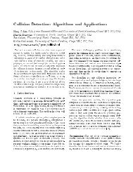
(a) (b) (c) (d) (e)<br />
Fig. 3. Visibility computation based on area subdivision: We highlight different cases that arise as we resolve visibility between two triangle<br />
primitives (shown in red and blue) from the apex of the frustum. In cases (a)-(b) the quadtree is refined based on the intersection depth associated<br />
with the outermost frustum and compared with the triangles. However, in cases (c)-(e) the outermost frustum has to be sub-divided into sub-frusta<br />
and each of them is compared separately.<br />
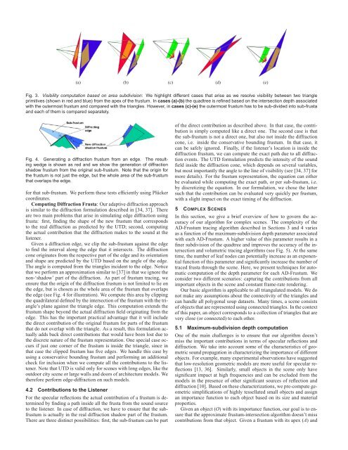
Fig. 4. Generating a diffraction frustum from an edge. The resulting<br />
wedge is shown as red and we show the generation of diffraction<br />
shadow frustum from the original sub-frustum. Note that the origin <strong>for</strong><br />
the frustum is not just the edge, but the whole area of the sub-frustum<br />
that overlaps the edge.<br />
<strong>for</strong> that sub-frustum. We per<strong>for</strong>m these tests efficiently using Plücker<br />
coordinates.<br />
Computing Diffraction Frusta: Our adaptive diffraction approach<br />
is similar to the diffraction <strong>for</strong>mulation described in [34, 37]. There<br />
are two main problems that arise in simulating edge diffraction using<br />
frusta: first, finding the shape of the new frustum that corresponds<br />
to the real diffraction as predicted by the UTD; second, computing<br />
the actual contribution that the diffraction makes to the sound at the<br />
listener.<br />
Given a diffraction edge, we clip the sub-frustum against the edge<br />
to find the interval along the edge that it intersects. The diffraction<br />
cone originates from the respective part of the edge and its orientation<br />
and shape are predicted by the UTD based on the angle of the edge.<br />
The angle is computed from the triangles incident to the edge. Notice<br />
that we per<strong>for</strong>m an approximation similar to [37] in that we ignore the<br />
non-‘shadow’ part of the diffraction. As part of frustum tracing, we<br />
ensure that the origin of the diffraction frustum is not limited to lie on<br />
the edge, but is chosen as the whole area of the frustum that overlaps<br />
the edge (see Fig. 4 <strong>for</strong> illustration). We compute this area by clipping<br />
the quadrilateral defined by the intersection of the frustum with the triangle’s<br />
plane against the triangle edge. This computation extends the<br />
frustum shape beyond the actual diffraction field originating from the<br />
edge. This has the important practical advantage that it will include<br />
the direct contribution of the original frustum <strong>for</strong> parts of the frustum<br />
that do not overlap with the triangle. As a result, this <strong>for</strong>mulation actually<br />
adds back direct contributions that would have been lost due to<br />
the discrete nature of the frustum representation. One special case occurs<br />
if just one corner of the frustum is inside the triangle, since in<br />
that case the clipped frustum has five edges. We handle this case by<br />
using a conservative bounding frustum and per<strong>for</strong>ming an additional<br />
check <strong>for</strong> inclusion when we compute all the contributions to the listener.<br />
Note that UTD is valid only <strong>for</strong> scenes with long edges, like the<br />
outdoor city scene or large walls and doors of architecture models. We<br />
there<strong>for</strong>e per<strong>for</strong>m edge-diffraction on such models.<br />
4.2 Contributions to the Listener<br />
For the specular reflections the actual contribution of a frustum is determined<br />
by finding a path inside all the frusta from the sound source<br />
to the listener. In case of diffraction, we have to ensure that the subfrustum<br />
is actually in the real diffraction shadow part of the frustum.<br />
There are three distinct possibilities: first, the sub-frustum can be part<br />
of the direct contribution as described above. In that case, the contribution<br />
is simply computed like a direct one. The second case is that<br />
the sub-frustum is not a direct one, but also not inside the diffraction<br />
cone, i.e. inside the conservative bounding frustum. In that case, it<br />
can be safely ignored. Finally, if the listener’s location is inside the<br />
diffraction frustum, we can compute the exact path due to all diffraction<br />
events. The UTD <strong>for</strong>mulation predicts the intensity of the sound<br />
field inside the diffraction cone, which depends on several variables,<br />
but most importantly the angle to the line of visibility (see [34, 37] <strong>for</strong><br />
more details). For the frustum representation, the equation can either<br />
be evaluated while computing the exact path, or per sub-frustum, i.e.<br />
by discretizing the equation. In our <strong>for</strong>mulation, we chose the latter<br />
such that the contribution can be evaluated very quickly per frustum,<br />
with a slight impact on the exact timing of the diffraction.<br />
5 COMPLEX SCENES<br />
In this section, we give a brief overview of how to govern the accuracy<br />
of our algorithm <strong>for</strong> complex scenes. The complexity of the<br />
AD-<strong>Frustum</strong> tracing algorithm described in Sections 3 and 4 varies<br />
as a function of the maximum-subdivision depth parameter associated<br />
with each AD-<strong>Frustum</strong>. A higher value of this parameter results in a<br />
finer subdivision of the quadtree and improves the accuracy of the intersection<br />
and volumetric tracing algorithms (see Fig. 5). At the same<br />
time, the number of leaf nodes can potentially increase as an exponential<br />
function of this parameter and significantly increase the number of<br />
traced frusta through the scene. Here, we present techniques <strong>for</strong> automatic<br />
computation of the depth parameter <strong>for</strong> each AD-<strong>Frustum</strong>. We<br />
consider two different scenarios: capturing the contributions from all<br />
important objects in the scene and constant frame-rate rendering.<br />
Our basic algorithm is applicable to all triangulated models. We do<br />
not make any assumptions about the connectivity of the triangles and<br />
can handle all polygonal soup datasets. Many times, a scene consists<br />
of objects that are represented using connected triangles. In the context<br />
of this paper, an object corresponds to a collection of triangles that are<br />
very close (or connected) to each other.<br />
5.1 Maximum-subdivision depth computation<br />
One of the main challenges is to ensure that our algorithm doesn’t<br />
miss the important contributions in terms of specular reflections and<br />
diffraction. We take into account some of the characteristics of geometric<br />
sound propagation in characterizing the importance of different<br />
objects. For example, many experimental observations have suggested<br />
that low-resolution geometric models are more useful <strong>for</strong> specular reflections<br />
[13, 36]. Similarly, small objects in the scene only have<br />
significant impact at high frequencies and can be excluded from the<br />
models in the presence of other significant sources of reflection and<br />
diffraction [10]. Based on these characterizations, we pre-compute geometric<br />
simplifications of highly tessellated small objects and assign<br />
an importance function to each object based on its size and material<br />
properties.<br />
Given an object (O) with its importance function, our goal is to ensure<br />
that the approximate frustum-intersection algorithm doesn’t miss<br />
contributions from that object. Given a frustum with its apex (A) and