Adaptive Frustum Tracing for Interactive Sound Propagation

More documents

Recommendations

Info

(a) (b) (c) (d) (e) Fig. 3. Visibility computation based on area subdivision: We highlight different cases that arise as we resolve visibility between two triangle primitives (shown in red and blue) from the apex of the frustum. In cases (a)-(b) the quadtree is refined based on the intersection depth associated with the outermost frustum and compared with the triangles. However, in cases (c)-(e) the outermost frustum has to be sub-divided into sub-frusta and each of them is compared separately. Fig. 4. Generating a diffraction frustum from an edge. The resulting wedge is shown as red and we show the generation of diffraction shadow frustum from the original sub-frustum. Note that the origin for the frustum is not just the edge, but the whole area of the sub-frustum that overlaps the edge. for that sub-frustum. We perform these tests efficiently using Plücker coordinates. Computing Diffraction Frusta: Our adaptive diffraction approach is similar to the diffraction formulation described in [34, 37]. There are two main problems that arise in simulating edge diffraction using frusta: first, finding the shape of the new frustum that corresponds to the real diffraction as predicted by the UTD; second, computing the actual contribution that the diffraction makes to the sound at the listener. Given a diffraction edge, we clip the sub-frustum against the edge to find the interval along the edge that it intersects. The diffraction cone originates from the respective part of the edge and its orientation and shape are predicted by the UTD based on the angle of the edge. The angle is computed from the triangles incident to the edge. Notice that we perform an approximation similar to [37] in that we ignore the non-‘shadow’ part of the diffraction. As part of frustum tracing, we ensure that the origin of the diffraction frustum is not limited to lie on the edge, but is chosen as the whole area of the frustum that overlaps the edge (see Fig. 4 for illustration). We compute this area by clipping the quadrilateral defined by the intersection of the frustum with the triangle’s plane against the triangle edge. This computation extends the frustum shape beyond the actual diffraction field originating from the edge. This has the important practical advantage that it will include the direct contribution of the original frustum for parts of the frustum that do not overlap with the triangle. As a result, this formulation actually adds back direct contributions that would have been lost due to the discrete nature of the frustum representation. One special case occurs if just one corner of the frustum is inside the triangle, since in that case the clipped frustum has five edges. We handle this case by using a conservative bounding frustum and performing an additional check for inclusion when we compute all the contributions to the listener. Note that UTD is valid only for scenes with long edges, like the outdoor city scene or large walls and doors of architecture models. We therefore perform edge-diffraction on such models. 4.2 Contributions to the Listener For the specular reflections the actual contribution of a frustum is determined by finding a path inside all the frusta from the sound source to the listener. In case of diffraction, we have to ensure that the subfrustum is actually in the real diffraction shadow part of the frustum. There are three distinct possibilities: first, the sub-frustum can be part of the direct contribution as described above. In that case, the contribution is simply computed like a direct one. The second case is that the sub-frustum is not a direct one, but also not inside the diffraction cone, i.e. inside the conservative bounding frustum. In that case, it can be safely ignored. Finally, if the listener’s location is inside the diffraction frustum, we can compute the exact path due to all diffraction events. The UTD formulation predicts the intensity of the sound field inside the diffraction cone, which depends on several variables, but most importantly the angle to the line of visibility (see [34, 37] for more details). For the frustum representation, the equation can either be evaluated while computing the exact path, or per sub-frustum, i.e. by discretizing the equation. In our formulation, we chose the latter such that the contribution can be evaluated very quickly per frustum, with a slight impact on the exact timing of the diffraction. 5 COMPLEX SCENES In this section, we give a brief overview of how to govern the accuracy of our algorithm for complex scenes. The complexity of the AD-Frustum tracing algorithm described in Sections 3 and 4 varies as a function of the maximum-subdivision depth parameter associated with each AD-Frustum. A higher value of this parameter results in a finer subdivision of the quadtree and improves the accuracy of the intersection and volumetric tracing algorithms (see Fig. 5). At the same time, the number of leaf nodes can potentially increase as an exponential function of this parameter and significantly increase the number of traced frusta through the scene. Here, we present techniques for automatic computation of the depth parameter for each AD-Frustum. We consider two different scenarios: capturing the contributions from all important objects in the scene and constant frame-rate rendering. Our basic algorithm is applicable to all triangulated models. We do not make any assumptions about the connectivity of the triangles and can handle all polygonal soup datasets. Many times, a scene consists of objects that are represented using connected triangles. In the context of this paper, an object corresponds to a collection of triangles that are very close (or connected) to each other. 5.1 Maximum-subdivision depth computation One of the main challenges is to ensure that our algorithm doesn’t miss the important contributions in terms of specular reflections and diffraction. We take into account some of the characteristics of geometric sound propagation in characterizing the importance of different objects. For example, many experimental observations have suggested that low-resolution geometric models are more useful for specular reflections [13, 36]. Similarly, small objects in the scene only have significant impact at high frequencies and can be excluded from the models in the presence of other significant sources of reflection and diffraction [10]. Based on these characterizations, we pre-compute geometric simplifications of highly tessellated small objects and assign an importance function to each object based on its size and material properties. Given an object (O) with its importance function, our goal is to ensure that the approximate frustum-intersection algorithm doesn’t miss contributions from that object. Given a frustum with its apex (A) and
c○2009 IEEE. Reprinted, with permission, from IEEE TRANSACTION ON VISUALIZATION AND COMPUTER GRAPHICS, VOL. 14, NO. 6, NOVEMBER/DECEMBER 2008 (a) (b) (c) (d) (e) (f) Fig. 5. Beam tracing vs. uniform frustum tracing vs. adaptive frustum tracing: We show the relative accuracy of three different algorithm in this simple 2D model with only first-order reflections. (a) Reflected beams generated using exact beam tracing. (b)-(c) Reflected frusta generated with uniform frustum tracing for increased sampling: 2 2 samples per frustum and 2 4 samples per frustum. Uniform frustum tracing generates uniform number of samples in each frustum, independent of scene complexity. (d)-(e) Reflected frusta generated using AD-Frustum. We highlight the accuracy of the algorithm by using the values of 2 and 4 for maximum-subdivision depth parameter. (f) An augmented binary tree for the 2D case (equivalent to a quadtree in 3D) showing the adaptive frusta. Note that the adaptive algorithm only generates more frusta in the regions where the input primitives have a high curvature and reduces the propagation error. the plane of its quadtree (P), we compute a perspective projection of the bounding box of O on the P. Let’s denote the projection on P as o. Based on the size of o, we compute a bound on the size of leaf nodes of the quadtree such that the squares corresponding to the leaf nodes are inside o. If O has a high importance values attached to it, we ensure multiple leaf nodes of the quadtree are contained in o. We repeat this computation for all objects with high importance value in the scene. The maximum-subdivision depth parameter for that frustum is computed by considering the minimum size of the leaf nodes of the quadtree over all objects. Since we use a bounding box of O to compute the projection, our algorithm tends to be conservative. 5.2 Constant frame rate rendering In order to achieve target frame rate, we can bound the number of frusta that are traced through the scene. We first estimate the number of frustum that our algorithm can trace per second based on scene complexity, number of dynamic objects and sources. Given a bound on maximum number of frusta traced per second, we adjust the number of primary frusta that are traced from each source. Moreover, we use a larger value of the maximum depth parameter for the first few reflections and decrease this value for higher order reflections. We compute the first few reflections with higher accuracy by performing more adaptive subdivisions. We also perform adaptive subdivisions of a frustum based on its propagated distance. In this manner, our algorithm would compute more contributions from large objects in the scene, and tend to ignore contributions from relatively small objects that are not close to the source or the receiver. We can further improve the performance by using dynamic sorting and culling algorithms along with perceptual metrics [38]. 6 IMPLEMENTATION AND RESULTS In this section, we highlight the performance of our algorithm on different benchmarks, describe our audio rendering pipeline, and analyze its accuracy. Our simulations were run on a 2.66 GHz Intel Core 2 Duo machine with 2GB of memory. 6.1 Performance Results We perform geometric sound propagation using adaptive frustum tracing on many benchmarks. The complexity of our benchmarks ranges from a few hundred triangles to almost a million triangles. The performance results for adaptive frustum tracing and complexity of benchmarks are summarized in Table 1. These results are generated for a maximum sub-division depth of 3. 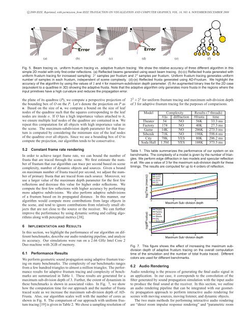Further, the extent of dynamism in these benchmarks is shown in associated video. In Fig. 7, we show how the computation time for our approach and the number of frusta traced scale as we increase the maximum sub-division depth of AD- Frusta. Also, our algorithm scales well with the number of cores as shown in Fig. 8. The comparison of our approach with uniform frustum tracing [19] is given in Table 2. We chose a sampling resolution of 2 3 × 2 3 for uniform frustum tracing and maximum sub-division depth of 3 for adaptive frustum tracing for the purposes of comparisons. Model Complexity Results (7 threads) #Δs diffraction #frusta time Theater 54 NO 56K 33.3 ms Factory 174 NO 40K 27.3 ms Game 14K NO 206K 273.3 ms Sibenik 71K NO 198K 598.6 ms City 78K YES 80K 206.2 ms Soda Hall 1.5M YES 108K 373.3 ms Table 1. This table summarizes the performance of our system on six benchmarks. The complexity of a model is given by the number of triangles. We perform edge diffraction in two models and specular reflection in all. We use a value of 3 for the maximum sub-division depth for these timings. The results are computed for up to 4 orders of reflection. log(Time (msecs)) log(#Frustua) 10 8 6 4 Theater Factory Game Sibenik City Soda Hall 2 2 3 4 5 Maximum Sub−division depth 16 14 12 10 Theater Factory Game Sibenik City Soda Hall 2 3 4 5 Maximum Sub−division depth Fig. 7. This figure shows the effect of increasing the maximum subdivision depth of adaptive frustum tracing on the overall computation time of the simulation and the number of total frusta traced. Different colors are used for different benchmarks. 6.2 Audio Rendering Audio rendering is the process of generating the final audio signal in an application. In our case, it corresponds to the convolution of the filter generated by sound propagation simulation with the input audio to produce the final sound at the receiver. In this section, we outline an audio rendering pipeline that can be integrated with our geometric propagation approach to perform interactive audio rendering for scenes with moving sources, moving listener, and dynamic objects. The two main methods for performing interactive audio rendering are “direct room impulse response rendering” and “parametric room
Page 1 and 2: c○2009 IEEE. Reprinted, with perm
Page 3: c○2009 IEEE. Reprinted, with perm
Page 7 and 8: c○2009 IEEE. Reprinted, with perm

Adaptive Frustum Tracing for Interactive Sound Propagation

You also want an ePaper? Increase the reach of your titles

Delete template?

Save as template?