Adaptive Frustum Tracing for Interactive Sound Propagation
Adaptive Frustum Tracing for Interactive Sound Propagation
Adaptive Frustum Tracing for Interactive Sound Propagation

Create successful ePaper yourself
Turn your PDF publications into a flip-book with our unique Google optimized e-Paper software.
c○2009 IEEE. Reprinted, with permission, from IEEE TRANSACTION ON VISUALIZATION AND COMPUTER GRAPHICS, VOL. 14, NO. 6, NOVEMBER/DECEMBER 2008<br />
A P<br />
(a) (b)<br />
Fig. 2. AD-<strong>Frustum</strong> Representation: (a) A frustum, represented by convex<br />
combination of four corner rays and apex A. (b) A hierarchically<br />
divided adaptive frustum. It is augmented with a quadtree structure,<br />
where P is the 2D plane of quadtree. We use two sets of colors to<br />
show different nodes. Each node stores auxiliary in<strong>for</strong>mation about corresponding<br />
sub-frusta.<br />
frusta. The scene is represented using a bounding volume hierarchy<br />
(BVH) of axis-aligned bounding boxes (AABBs). The leaf nodes of<br />
the BVH are triangle primitives and the intermediate nodes represent<br />
an AABB. For dynamic scenes, the BVH is updated at each frame<br />
[39, 21, 43]. Given an AD-<strong>Frustum</strong>, we traverse the BVH from the<br />
root node to per<strong>for</strong>m these tests.<br />
Intersection with AABBs: The intersection of an AD-<strong>Frustum</strong><br />
with an AABB is per<strong>for</strong>med by intersecting the four corner rays of<br />
the root node of the quadtree with the AABB, as described in [26]. If<br />
an AABB partially or fully overlaps with the frustum, we apply the algorithm<br />
recursively to the children of the AABB. The quadtree is not<br />
modified during this traversal.<br />
Intersection with primitives: As a frustum traverses the BVH,<br />
we compute intersections with each triangle corresponding to the leaf<br />
nodes of the BVH. We only per<strong>for</strong>m these tests to classify the node as<br />
completely-inside, completely-outside or partially-intersecting. This<br />
is illustrated in Fig. 3, where we show the completely-outside regions<br />
in green and completely-inside regions in orange. This intersection<br />
test can be per<strong>for</strong>med efficiently by using the Plücker coordinate<br />
representation [31] <strong>for</strong> the triangle edges and four corner rays. The<br />
Plücker coordinate representation efficiently determines, based on an<br />
assumed orientation of edges, whether the sub-frustum is completely<br />
inside, outside or partially intersecting the primitive. This test is conservative<br />
and may conclude that a node is partially intersecting, even<br />
if it is completely-outside. If the frustum is classified as partiallyintersecting<br />
with the primitives, we sub-divide that quadtree node,<br />
generate four new sub-frusta, and per<strong>for</strong>m the intersection test recursively.<br />
The maximum-subdivision depth parameter imposes a bound<br />
on the depth of the quadtree. Each leaf node of the quadtree is classified<br />
as completely-outside or completely-inside.<br />
3.3 Visible Surface Approximation<br />
A key component of the traversal algorithm is the computation of the<br />
visible primitives associated with each leaf node sub-frustum. We use<br />
an area-subdivision technique, similar to classic Warnock’s algorithm<br />
[41], to compute the visible primitives. Our algorithm associates intersection<br />
depth values of four corner rays with each leaf node of the<br />
quadtree as well as the id of the corresponding triangle. Moreover,<br />
we compute the minimum and maximum depth <strong>for</strong> each intermediate<br />
node of the triangle, that represents the extent of triangles that partially<br />
overlap with its frustum. The depth in<strong>for</strong>mation of all the nodes<br />
is updated whenever we per<strong>for</strong>m intersection computations with a new<br />
triangle primitive.<br />
In order to highlight the basic subdivision algorithm, we consider<br />
the case of two triangles in the scene shown as red and blue in Fig. 3.<br />
In this example, the projections of the triangles on the quadtree plane<br />
overlap. We illustrate different cases that can arise based on the relative<br />
ordering and orientation of two triangles. The basic operation<br />
compares the depths of corner rays associated with the frustum and<br />
updates the node with the depth of the closer ray (as shown in Fig.<br />
3(a)). If we cannot resolve the closest depth (see Fig. 3(d)), we apply<br />
the algorithm recursively to its children (shown in orange). Fig.<br />
3(b) shows the comparison between a partially-intersecting node with<br />
a completely-inside node. If the completely-inside node is closer, i.e.,<br />
all the corner rays of the completely-inside node are closer than the<br />
minimum depth of the corner rays of the partially-intersecting node,<br />
then the quadtree is updated with the completely-inside node. Otherwise,<br />
we apply the algorithm recursively to their children as in Fig.<br />
3(e). Lastly, in Fig. 3(c), both the nodes are partially-intersecting and<br />
we apply the algorithm recursively on their children.<br />
This approach can be easily generalized to handle all the triangles<br />
that overlap with an AD-<strong>Frustum</strong>. At any stage, the algorithm maintains<br />
the depth values based on intersection with all the primitives traversed<br />
so far. As we per<strong>for</strong>m intersection computations with a new<br />
primitive, we update the intersection depth values by comparing the<br />
previous values stored in the quadtree. The accuracy of our algorithm<br />
is governed by the resolution of the leaf nodes of the quadtree, which<br />
is based on the maximum-subdivision depth parameter associated with<br />
each AD-<strong>Frustum</strong>.<br />
3.4 Nodes Reduction<br />
We per<strong>for</strong>m an optimization step to reduce the number of frusta. This<br />
step is per<strong>for</strong>med in a bottom up manner, after AD-<strong>Frustum</strong> finishes<br />
the scene traversal. We look at the children of a node. Since, each<br />
child shares atleast one corner-ray with its siblings, we compare the<br />
depths of these corner-rays. Based on the difference in depth values,<br />
the normals of the surfaces the sub-frustum intersects, and the acoustic<br />
properties of those surfaces we collapse the children nodes into the<br />
parent node. Thus, we can easily combine the children nodes in the<br />
quadtree that hit the same plane with similar acoustic properties. Such<br />
an approach can also be used to combine children nodes that intersect<br />
slightly different surfaces.<br />
4 ENUMERATING PROPAGATION PATHS<br />
In the previous section, we described the AD-<strong>Frustum</strong> representation<br />
and presented an efficient algorithm to compute its intersection and<br />
visibility with the scene primitives. In this section, we present algorithms<br />
to trace the frusta through the scene, and compute reflection<br />
and diffraction frusta. We start the simulation by computing initial<br />
frusta around a sound source in quasi-uni<strong>for</strong>m fashion [27] and per<strong>for</strong>m<br />
adaptive subdivision based on the intersection tests. Ultimately,<br />
the sub-frusta corresponding to the leaf nodes of the quadtree are used<br />
to compute reflection and diffraction frusta.<br />
Specular Reflections: Once a frustum has completely traced a<br />
scene, we consider all the leaf nodes within its quadtree and compute<br />
a reflection frustum <strong>for</strong> all completely-intersecting leaf nodes. The<br />
corner rays of sub-frustum associated with the leaf nodes are reflected<br />
(see Fig. 5) at the primitive hit by that sub-frustum. The convex combination<br />
of the reflected corner rays creates the parent frustum <strong>for</strong> the<br />
reflection AD-<strong>Frustum</strong>.<br />
4.1 Edge Diffraction<br />
Diffraction happens when a sound wave hits an object whose size is<br />
the same order of magnitude as its wavelength, causing the wave to<br />
scatter. Our <strong>for</strong>mulation of diffraction is based on the uni<strong>for</strong>m theory<br />
of diffraction (UTD) [15], which predicts that a sound wave hitting an<br />
edge between the primitives is scattered in a cone. The half-angle of<br />
the cone is determined by the angle that the ray hits the edge. The basic<br />
ray-frustum tracing algorithm can compute edge diffraction based on<br />
UTD [34]. This involves identifying diffraction edges as part of a<br />
pre-process and computing diffraction paths using frusta tracing. In<br />
this section, we extend the approach described in [34] to handle AD-<br />
Frusta.<br />
Finding diffracting edges: In a given scene, only a subset of the<br />
edges are diffraction edges. For example, any planar rectangle is represented<br />
by two triangles sharing an edge, but that edge cannot result in<br />
diffraction. Most edges in a model are shared by at least two triangles.<br />
As part of a pre-computation step, we represent the adjacency in<strong>for</strong>mation<br />
using an edge-based data structure that associates all edges that<br />
can result in diffraction with its incident triangles. As part of the tracing<br />
algorithm, we compute all triangles that intersect a sub-frustum.<br />
Next, we check whether the sub-frustum intersects any of the edges<br />
of that triangle and based on that update the list of diffracting edges