Link to Fulltext

6 Calibration
6.1 Time calibration
During the first calibration phase, right after deployment at the South Pole, a YAG laser was
used to measure all the time delays due to different cable-lengths and transit times in the
PMs
) which have to be subtracted from subsequent leading-edge measurements. An optical fiber
(
ending at an isotropizing nylon ball right below each OM was used to send light from the surface
with the YAG-laser. The data thus acquired was then used to make the in-situ time-calibration
of the detector. The distance between the nylon ball and the OM is typically less than a meter
(much less than one scattering length in ice), so that we can safely assume that all hits are direct
(unscattered).
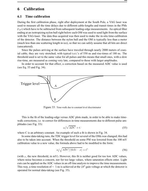
Since the pulses arriving at the surface have traveled through nearly 2000 meters of coaxial
cable, they are very stretched, with typical t.o.t.’s of 550 ns and rise-times of 180 ns. The
threshold used is set to the same value for all pulses and this means that small ones, with a slow
rise-time, are measured as coming very late, compared to those with larger amplitudes.
In order to account for that effect, a correction based on the measured ADC value is used
(see Eq. 55 and Fig. 34).
Trigger level
A
B
Figure 33: Time-walk due to constant level discriminator
This is the fit of the leading-edge versus ADC plots made, in order to be able to make timewalk
corrections, i.e. to correct for differences in time measurements due to different pulse amplitudes
(see Fig.
£
33):
¡£¢ ¢
(55)
where C is an arbitrary constant. An example of such a fit is shown in Fig. 34.
In some data-taking runs, the TDC trigger level for several of the OMs was changed; this had
also to be taken into account. When the threshold on some PM was lowered from the 100 mV
calibration value to a new value, the formula above had to be modified to the form:
¢
£ ¢ ¡
¡
¡ ¢
(with
, the new threshold, in mV). However, this fit is neither good for too low ADC values,
where noise becomes a concern, nor for too large values, where saturation effects enter. Light
cuts can be applied on the ADC values in an off-line analysis to improve the time measurements.
This way, a time resolution ¥ of ns is achieved at the ¡ § gain voltage at which the detector is
operated for normal data-taking (see Fig. 35).
44
(56)