Link to Fulltext

That a precision of 5 ns is required for an efficient use of the detector is shown in section 9,
where a comparison is made between the results of Monte Carlo simulation analyses at this measured
5 ns resolution and at 5 ns resolution with added systematic errors of ¥ 15 ns resolution
in each module.
6.2 Position calibration
6.2.1 Laser positioning
Measurements
In order to measure the OM positions and the ice properties, calibration data was taken while
sending out light pulses with a YAG-laser at the surface. That light was led by an optical fiber
to a diffusive nylon sphere right below an optical module. There were two such fibers per OM.
A specific laser-module was installed 10 meters below OM16 (module 16 on string 1) for the
same purpose, and a few specially designed LED modules were put at various locations inside
the detector. The main goals were to study the optical properties of the ice at the depths at which
the detector was buried, and — what concerns us here — to make an as accurate as possible
position calibration of the detector.
The laser module contained a¤ laser pulsed at a rate of 6 Hz, which made it possible to send
light pulses strong enough to reach modules at large distances, as opposed to the surface-based
sources. This laser gave a wavelength of 337 nm, for which the attenuation length in the ice is
very large.
From the data taken with it, only the last three data-runs (158–160) were found to be usable, the
remaining ones containing too few events.
The data-taking conditions were as follows:
The voltage of OM16 at a gain of ¡ § is 1680 V.
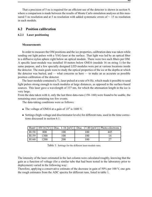
Settings (high-voltage and discriminator levels) for different runs, used in the time corrections
discussed in section 6.1:
Run# HV16 [V] Disc. 1-16 [mV] Disc. 17-80 [mV] Photo-electrons
R158 800 100 100 445
R159 1300 100 100 14
R160 1200 200 100 27
Table 1: Settings for the different laser-module runs.
The intensity of the laser estimated in the last column were calculated roughly, knowing that the
gain as a function of voltage (for a similar tube that had been tested in the laboratory prior to
deployment) varied in the following way:
Therefore, applying a conservative estimate of the decrease in gain of 50% per 100 V, one gets
the rough estimates from the ADC spectra for different runs, listed in table 1.
46