2012 METU Lecture 5 Control of Smart Systems - Department of ...

•
•
•
•
•
•
Lecture 1: Introduction to Smart Materials and
Systems
Lecture 2: Sensor technologies for smart systems
and their evaluation criteria.
Lecture 3: Actuator technologies for smart
systems and their evaluation criteria.
Lecture 4: Piezoelectric Materials and their
Applications.
Lecture 5: Control System Technologies.
Lecture 6: Smart System Applications.
S. Eswar Prasad,
Adjunct Professor, Department of Mechanical & Industrial Engineering,
Chairman, Piemades Inc,
⎋ Piemades, Inc.
1

Control Technologies
for Smart Systems
S. Eswar Prasad,
Adjunct Professor, Department of Mechanical & Industrial Engineering,
Chairman, Piemades Inc,
⎋ Piemades, Inc.
2

Control Technologies for Smart Systems
• Control Systems Overview
Open loop and closed loop systems
• Control System Characteristics
Steady State, Transient Response and Stability
• Controller Operation
Proportional, Compensated
• Digital Control Systems
Control algorithms, implementation, hardware
• Control System Design
3
3

Control Systems Overview
•
•
•
•
Deals with influencing the behaviour of dynamic systems
Interdisciplinary field, which originated in engineering and
mathematics, and evolved into use by the social sciences, like
psychology, sociology, criminology and in financial systems.
Control systems have four basic functions; Measure,
Compare, Compute, and Correct.
These four functions are completed by three elements;
Sensors, Actuators, Control System. In a smart system, these
three elements are typically contained in one unit.
4

Control Systems Overview
Definition of a Smart System
5

Control Systems Overview
Historical
Feedback control (Bode,1945)
Theory of Stochastic Processes (Weiner, 1930)
Root Locus Theory (Evans, 1948)
Modern Control (1950s, Kalman, Bellman, Pontryagin)
• Root locus theory remains an important technique today.
• Suitable for design and stability analysis.
Root locus analysis is a graphical method for examining how the
roots of a system change with variation of a certain system
parameter, commonly the gain of a feedback system. This is a
technique used in the field of control systems developed by Walter
R. Evans.
6

Control Systems Overview
Root locus approach
Assumption
The definition of the damping ratio and natural frequency
presumes that the overall feedback system is well approximated by
a second order system, that is, the system has a dominant pair of
poles.
Uses
• Determine the stability of the system
• Design for the damping ratio and natural frequency of a
feedback system.
• Lag, lead, PI, PD and PID controllers can be designed
approximately with this technique.
7

Control Systems Overview
•
•
•
Example: cruise control of a car
Cruise Control is a device designed to
maintain vehicle speed at a constant desired
or reference speed provided by the driver.
The controller is the cruise control, the plant
is the car, and the system is the car and the
cruise control. The system output is the car's
speed, and the control itself is the engine's
throttle position which determines how
much power the engine generates.
8

Control System Technology
•
•
Method-1. Implement cruise control by simply locking the
throttle position when the driver engages cruise control.
However, if the cruise control is engaged on a stretch of flat
road, then the car will travel slower going uphill and faster
when going downhill.
Method-2. Use the system output (the car's speed) to
control the throttle position. As a result, the controller can
compensate for changes acting on the car, like a change in
the slope of the road.
9

Control Systems Overview
Types of Control systems
• Open Loop Control
• Closed Loop Control
10

Open Loop System
•
•
Reference
Input
Controller
Actuating
Signal
Controlled Process
(Plant)
General block diagram of an open-loop system
Controlled
Variable
(output)
An open-loop controller is often used in simple processes
because of its simplicity and low cost, especially in systems
where feedback is not critical
An open-loop controller, also called a non-feedback controller,
is a type of controller that computes its input into a system
using only the current state and its model of the system.
11

Open Loop System
Reference
Input
•
•
Controller
Actuating
Signal
Controlled Process
(Plant)
General block diagram of an open-loop system
Controlled
Variable
(output)
A characteristic of the open-loop controller is that it
does not use feedback to determine if its output has
achieved the desired goal of the input. This means that
the system does not observe the output of the
processes that it is controlling.
It also may not compensate for disturbances in the
system.
12

Open Loop System
Reference
Input
•
Controller
Actuating
Signal
Controlled Process
(Plant)
General block diagram of an open-loop system
Controlled
Variable
(output)
Typical examples: Washing Machine, for which the length of
machine wash time is entirely dependent on the judgment
and estimation of the human operator. Some Irrigation
Sprinklers are programmed to turn on/off at set times. It
does not measure soil moisture as a form of feedback. Even if
rain is pouring down on the lawn, the sprinkler system would
activate on schedule, wasting water.
13

Closed Loop System
Reference
Input
Error
Detector
+ -
Feedback
Signal
Error
Signal
Controller
Actuating
Signal
Feedback Path Elements
Controlled
Process
(Plant)
General block diagram of a closed-loop control system
Controlled
Variable
(output)
A closed-loop controller uses feedback to control states or outputs
of a dynamical system. Its name comes from the information path in
the system: Process inputs have an effect on the process outputs,
which is measured with sensors and processed by the controller;
the result (the control signal) is used as input to the process, closing
the loop.
14

Error
Detector
Closed Loop System
Reference
Input
Signal
Controller
Closed-loop controllers have the following advantages over open-loop
controllers:
• Reduce error (eliminating the error)
• Reduce sensitivity or Enhance robustness
• Disturbance rejection or elimination
• Improve dynamic performance or adjust the transient response (such as
reduce time constant) rejection (such as unmeasured friction in a motor)
+ -
Feedback
Signal
• unstable processes can be stabilized
• improved reference tracking performance
Error
Actuating
Signal
Feedback Path Elements
Controlled
Process
(Plant)
General block diagram of a closed-loop control system
Controlled
Variable
15

Closed Loop System
•
•
•
•
•
Examples of Closed Loop Systems
An air conditioning system or a heating system in a house.
The mouse on a computer
A joystick on a video game
Reference
Input
Controller
The speed control (cruise control) on an automobile.
+ -
Feedback
Signal
Error
Error
Signal
Actuating
Signal
Feedback Path Elements
Controlled
Process
(Plant)
General block diagram of a closed-loop control system
Controlled
Variabl
16

Closed Loop System
Sensor
The output of the system y(t) is fed back through a sensor
measurement F to the reference value r(t). The controller C
then takes the error e (difference) between the reference and the
output to change the inputs u to the system under control P.
This kind of controller is a closed-loop controller or feedback
controller.
This is called a single-input-single-output (SISO) control system;
MIMO (i.e., Multi-Input-Multi-Output) systems, with more than one
input/output, are common. In such cases variables are represented
through vectors instead of simple scalar values.
17

Closed Loop System
Sensor
If we assume the controller C, the plant P, and the sensor F are linear and timeinvariant
(i.e., elements of their transfer function C(s), P(s), and F(s) do not depend on
time), the systems above can be analyzed using the Laplace transform on the
variables. This gives the following relations:
Solving for Y(s) in terms of R(s) gives:
18

Closed Loop System
The expression
Sensor
is referred to as the closed-loop transfer function of the system. The numerator is
the forward (open-loop) gain from r to y, and the denominator is one plus the gain in
going around the feedback loop, the so-called loop gain. If , i.e., it has a large norm
with each value of s, and if ,
then Y(s) is approximately equal to R(s) and the output closely tracks the reference
input.
19

Selection of a Control System
Trade-offs
An open-loop
system
• Simplicity and low cost
• Complexity and higher cost
A closed-loop
system
20

Elements of Control Systems Response Characteristics
• Steady State Response
• Transient Response
• Stability
21

Elements of Control Systems Response Characteristics
Steady State Response is defined as the output of the plant.
Difference between final value and the desired value is known as
the steady-state error.
Amplitude
Input Command
Overshoot
Transient Response
Time
Steady State Response
Steady State
Error
22

Elements of Control Systems Response Characteristics
Transient Response is defined as the change undergone by plant from
time input is applied to the time taken to reach steady state. The ideal
situation is to reach the final state accurately and in as little time as
possible.
Four parameters define the transient response.
Amplitude
Input Command
Overshoot
Transient Response
Time
Steady State Response
Steady State
Error
23

Elements of Control Systems Response Characteristics
Amplitude
Input Command
Overshoot
Transient Response
Settling time, ts, is the time it takes output to settle within a specified boundary
typically 2%).
Rise time, tr, is the time it takes for the output to change from 10% to 90% of final
value.
Peak time, tp, is the time to reach the vicinity of set point, and usually the largest,
peak.
Overshoot, Mp, is the amount that the peak exceeds the steady state value at the
peak time. generally expressed as a percentage of the final steady state value.
Time
Steady State Response
Steady State
Error
24

Elements of Control Systems Response Characteristics
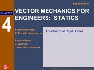
• Stability is defined as the ability of a control system to
achieve its goal without going into oscillation.
• The total response of a control system is a combination
of the natural response, totally governed by the plant,
and the forced response, typically governed by the
controller.
• It is a mandatory requirement that a control system be
stable.
25

Open loop
Closed Loop
Step response of a control system
26

Elements of Control Systems Response Characteristics
Considering a second order system, we can derive expressions for
the terms using the pole location parameters ζ and ωn.
27

Elements of Control Systems Response Characteristics
Considering a second order system, we can derive expressions for
the terms using the pole location parameters ζ and ωn.
28

Controller Operation
Controller provides a means to allow the output of a system to
track the input. Using frequency domain analysis methods, the
transfer function can be expressed as,
Ideally , Y(s)=1, and the output tracks input perfectly. Controllers
are broadly classified into two types.
• Proportional Controllers
• Compensated Controllers
29

Proportional Controllers
In the proportional control algorithm, the controller output is
proportional to the error signal, which is the difference between
the set point and the process variable. In other words, the output
of a proportional controller is the multiplication product of the
error signal and the proportional gain.
This can be mathematically expressed as
where
Pout: Output of the proportional controller
Kp: Proportional gain
e(t): Instantaneous process error at time 't'. e(t) = SP − PV
SP: Set point
PV: Process variable
30

Compensated Controllers
• Compensation is a technique used to change the root locus so
that it passes through a desired pole position.
• This process involves the selective positioning of additional
poles and zeros into the overall response of the system.
• Compensation can be used to improve both the steady state
error and the transient response.
• Most controllers now are implemented digitally.
31

PID Controllers
A proportional–integral–derivative controller (PID controller) is a
generic control loop feedback mechanism (controller) widely used
in industrial control systems – a PID is the most commonly used
feedback controller. A PID controller calculates an "error" value as
the difference between a measured process variable and a desired
set point. The controller attempts to minimize the error by
adjusting the process control inputs.
u(t)
+
-
P
+
e(t)
+
∑ ∑ Plant/Process
I
D
+
y(t)
32

PID Controllers
• The PID controller calculation (algorithm) involves three separate constant
parameters, the proportional, the integral and derivative values, denoted P, I, and
D.
• These values can be interpreted in terms of time: P depends on the present
error, I on the accumulation of past errors, and D is a prediction of future
errors, based on current rate of change. The weighted sum of these three
actions is used to adjust the process via a control element.
• In the absence of knowledge of the underlying process, a PID controller is the
best controller. By tuning the three parameters in the PID controller algorithm,
the controller can provide control action designed for specific process
requirements.
• The the use of the PID algorithm for control does not guarantee optimal
control of the system or system stability.
CONTROL SYSTEMS, ROBOTICS, AND AUTOMATION – Vol. II - PID Control - Araki M.
http://en.wikipedia.org/wiki/Special:BookSources/9-780863412998
http://en.wikipedia.org/wiki/PI_controller#PI_controller
33

PID Controllers
In PID control the sum of its three correcting terms constitutes
the manipulated variable (MV). The proportional, integral, and
derivative terms are summed to calculate the output of the PID
controller. Defining u(t) as the controller output, the final form of
the PID algorithm is:
where
Kp : Proportional gain, a tuning parameter
Ki : Integral gain, a tuning parameter
Kd : Derivative gain, a tuning parameter
e : Error = SP − PV
t : Time or instantaneous time (the present)
34

PID Controllers
u(t)
+
P
+
e(t)
+
∑ ∑ Plant/Process
-
Parameter Rise Time Overshoot Settling Time
I
D
+
Steady-state
Error
y(t)
Stability
Kp Decrease Increase Small Change Decrease Degrade
Ki Decrease Increase Increase
Kd
Small Increase
Small
decrease
Small
decrease
Large
decrease
No effect in
theory
Ang, K.H., Chong, G.C.Y., and Li, Y. (2005) PID control system analysis, design, and technology.
IEEE Transactions on Control Systems Technology, 13 (4). pp. 559-576.
Jinghua Zhong (2006). PID Controller Tuning: A Short Tutorial.
Degrade
Improve if Kd
is small
35

PID Controllers
Open Loop step response (OL) Proportional Control (P) Proportional Derivative control (PD)
http://www.engin.umich.edu/group/ctm/PID/PID.html
Proportional Integral control (PI) Proportional-Integral-Derivative Control (PID)
36

PID Controllers - Limitations
• While PID controllers are applicable to many control problems,
and often perform satisfactorily without any improvements or
even tuning, they can perform poorly in some applications, and
do not in general provide optimal control.
• The fundamental difficulty with PID control is that it is a
feedback system, with constant parameters, and no direct
knowledge of the process, and thus overall performance is
reactive and a compromise.
37

PID Controllers - Limitations
• PID controllers, when used alone, can give poor performance
when the PID loop gains must be reduced so that the control
system does not overshoot, oscillate or hunt about the control
set point value.
• PID controllers have difficulties in the presence of nonlinearities,
may trade-off regulation versus response time, do not
react to changing process behaviour (say, the process changes
after it has warmed up), and have lag in responding to large
disturbances.
38

PID Controllers - Limitations & Solutions
• While PID control is the best controller with no model of the
process, better performance can be obtained by incorporating a
model of the process.
• The most significant improvement is to incorporate feedforward
control with knowledge about the system, and using
the PID only to control error.
• PIDs can also be modified in more minor ways, such as by
changing the parameters (either gain scheduling in different use
cases or adaptively modifying them based on performance),
improving measurement (higher sampling rate, precision, and
accuracy, and low-pass filtering if necessary), or cascading
multiple PID controllers.
39

Design of Control Systems - Process
Objectives
• To aid the product or process - the mechanism, the robot, the
chemical plant, the aircraft, etc to do its job.
• Optimize performance for stability, disturbance regulation,
tracking accuracy or reduction of the effects of parameter
variations.
40

Design of Control Systems - Process Steps
• Understand the process and its performance requirements.
• Select the number and type of sensor(s) considering the
location, technology and noise.
• Select the number and types of actuators considering the
location, technology, noise and power.
• Develop a linear model of the process, actuator and sensor.
• Design a compensated controller.
• Test, modify and re-test.
Feedback Control of dynamic Systems, Franklin, Powell and Emami-Naeini, 2006 Prentice-Hall.
41

Design of Control Systems - Analogue Systems
• Typically consist of an operational amplifier based active filter
with either lowpass or bandpass characteristics.
• Responses are governed by available filter types - Bessel,
Chebyshev and Butterworth.
• Low pass compensators also known as lag compensators or PI
(Proportional Integral) controllers.
• Bandpass networks are referred as lead-lag compensators or
PID controllers.
42

Design of Control Systems - Digital Systems
Desired
Response
+
+
-
Error
Digital
Controller
Response
Analogueto-Digital
Converter
Digital-to-
Analogue
COnverter
Feedback
Sensor
Response
Digital Systems typically mimic analogue varieties.
Plant
Response
Exception is that of data conversion of both controller output and
feedback signals.
Output
Response
43

Design of Control Systems - Digital Systems
Advantages
• Easier implementation, since responses can be programmed.
• Parameter drift is eliminated.
• Changes are easy and almost always require no circuit
modifications.
• Reductions in size, power, weight and cost.
• Reliability (easier testing and verification regimes).
44

Design of Control Systems - Digital Systems
Digital controllers, in addition to PID, provide additional
algorithms.
• Notch Filter
Notch filters are used to control mechanical resonances in a
plant.
• Dead Beat Controller
Deadbeat controller provides very short settling times in a
control system by replacing all of the poles in the systems with
poles at the origin.
• Adaptive Filter
Adaptive filters are useful when plant response cannot be
determined due to insufficient information or if it is subjected
to time varying change. Can also be used to characterize an
unknown plant.
45

Algorithm Implementation Considerations
Digital processing systems operate using sampled data instead of
continuous data as is used in analogue systems. Mathematically,
differential equations are used to model DSP functions.
A DSP contains a MAC or Multiply-Accumulate Instruction. This
allows the multiplication of one variable by another and the
subsequent summation of the resulting product with the
accumulator, all operations occurring in one processor cycle.
This fact makes DSP processors ideal candidates for medium to
high performance embedded control applications requiring
computation intensive processing.
Two of the most important building blocks of DSP are FIT and the
IIR filters.
46

Algorithm Implementation Considerations - FIR Filter
"FIR" means "Finite Impulse Response".
They can easily be designed to be "linear phase" (and usually are).
Put simply, linear-phase filters delay the input signal but don’t
distort its phase.
They are simple to implement. On most DSP microprocessors, the
FIR calculation can be done by looping a single instruction.
They are suited to multi-rate applications.
FIR Filters are feedforward filters where the output values are a
function of a finite number of past input values.
FIR filters tend to be used where pass band characteristics are
specified. These include the start and end of passband and ripple.
47

Algorithm Implementation Considerations - IIR Filter
IIR means "Infinite Impulse Response".
The impulse response is "infinite" because there is feedback in the
filter.
IIR filters can achieve a given filtering characteristic using less
memory and calculations than a similar FIR filter.
They are however more susceptible to problems of finite-length
arithmetic, such as noise generated by calculations, and limit cycles.
They are harder (slower) to implement using fixed-point
arithmetic.
They don't offer the computational advantages of FIR filters for
multirate (decimation and interpolation) applications.
48

Algorithm Implementation Considerations - Filter Comparison
IIR FIR
More efficient Less efficient
Analog equivalent No analog equivalent
May be unstable Always stable
Non-liner phase response Linear phase response
No efficiency gained by
decimation
Decimation increases
efficiency
49

Control System Hardware Implementation
Sensor
Input
condition
Desired
Response
Input
• The heart of the controller is the processor.
• It is often single chip device.
Digital
Signal
Processor
Plant
• There are three types:
microcontrollers, microprocessors
DSPs.
Code/Data
Memory
Output
condition
Functional Diagram of a DSP based Controller
Driver
50

Control System Hardware Implementation - Microcontrollers
• Microcontrollers are single chip devices with a low to medium
performance core, a basic for of I/O (input/output), memory.
• Processors do not contain any inherent mathematical type
functions. complex operations must be performed with simpler
arithmetic, logical, and data move functions.
• Can be used in low performance applications. best suited for
high volume, simple function control systems that do not
demand high performance.
• Cost is relatively low.
• Examples are: PIC family, Motorola 68H series and Intel 8051
series.
51

Control System Hardware Implementation - Microprocessors
• Microprocessors are generally low to high performance devices
that rely on external I/O peripherals and memory for proper
operation.
• Operational speeds are higher than microcontrollers.
• More complex instructions are available as well as some floating
point arithmetic on the chip or as a processor.
• can be used in low to moderate performance control systems,
including ancillary functions such as human-machine interfaces.
• Cost is moderate to high.
• Examples are Motorola’s 68000 and Power PC families; AMD
Opteron family, Cypress Semiconductor PSoC family and Intel
i960 family.
52

Control System Hardware Implementation - DSPs
• DSPs are high performance processors, optimized for
computational efficiency.
• built in ports for interfacing with ADCs and DACs and other
processors.
• Data can be represented in fixed point or floating point
formats. Programs can be loaded from eternal memory.
• Handle moderate to high performance control systems.
• Cost is low to moderate.
• Examples are Analog Devices 21xx family, Texas Instruments
C6000 family and Motorola 96000 family.
53

Control System Hardware Implementation - Factors
• Sensor input
dynamic range, sampling rate, number of sensor inputs
interface, polled or interrupt driven.
• Control algorithm
fixed point or floating point, computational performance
requirements, data storage requirement, program storage
requirement.
• Controller output considerations
Same as sensor input.
• Cost and Schedule
COST versus product development.
54

Control System Hardware Implementation - Typical Plant Parameters
Parameter Sensing Method
Position
Speed
Acceleration
Potentiometer (linear or angular)
LVDT (Linear)
Resolver (Angular)
Optical Encoder (Linear or Angular)
Tachometer (RPM to voltage)
Hall Effect (Frequency)
Optical Encoder (Frequency)
Piezoelectric Accelerometer
Strain Gage Accelerometer
55

Control System Hardware Implementation - Typical Plant Parameters
Parameter Sensing Method
Temperature
Pressure
Force
Flow Rate
Thermocouple
Semiconductor Junction
Thermisotr
Strain Gage
Piezoelectric Force Transducer
Strain Gage
Piezoelectric Force Transducer
Differential Pressure
Impeller (Frequency)
Thermal (Differential temperature)
56

Control System Hardware Implementation - Factors
LNA
BPF
DSP Input Schematic Diagram
VGA
ADC
VGA Control
from DSP
• Input Signal Conditioning
Amplification of sensor signals, filtered, variable gain amplifier for
adjustment, analogue to digital converter and interface to DSP.
• Controller Response
local control - no operator inout
control by another processor through a port - interactive
control
Data to
DSP
57

Control System Hardware Implementation - Factors
Data
from DSP
Control
from DSP
DAC
PWM
DSP Output Schematic Diagram
Plant
Drive
• Controller Output
Output signal is converted back to analogue signal with a DAC,
filtered, fed to power amplifier.
LPF
Buffer
PA
PA
Plant
Drive
58

Control System Hardware Implementation - Method
• Translate the system requirements into a design specification
• Translate the design specification into a functional block
diagram.
• Optimize the block diagram.
• Translate the block diagram into a mathematical model.
• Optimize the mathematical model.
59

Control System Hardware Implementation - Block Diagram
60

Control System Hardware Implementation - Case Studies
• Computer Hard disk Control System.
This case study demonstrates the ability to perform classical
digital control design by going through the design of a
computer hard-disk read/write head position controller.
• Automobile Active Suspension System.
The vehicle suspension system is responsible for driving
comfort and safety as the suspension caries the vehicle body
and transmits all forces between the body and the road. By
adding an active suspension comfort and safety are
considerably improved compared to suspension setups with
fixed properties.
61

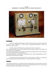
Hard Disc Drive Description
62

Hard Disc Drive Description
• Disk read/write heads are the small parts of a disk drive, that move
above the disk platter and transform platter's magnetic field into
electrical current (read the disk) or vice versa – transform electrical
current into magnetic field (write the disk)
• They are high-precision, high- performance machines produced in very
high volumes and sold at relatively low cost.
63

Performance of a Hard Disc Drive
There are three ways to measure the performance of a hard disk:
• Data Rate – The data rate is the number of bytes per second
that the drive can deliver to the CPU. Rates between 5 and 40
megabytes per second are common.
• Seek Time – The seek time is the amount of time between
when the CPU requests a file and when the first byte of the file
is sent to the CPU. Times between 10 and 20 milliseconds are
common.
• Capacity - The other important parameter is the capacity of the
drive, which is the number of bytes it can hold.
64

Hard Disc Drive Description
• In a hard drive, the heads 'fly' above the disk surface with clearance of as
little as 3 nanometres. The "flying height" is constantly decreasing to
enable higher areal density. The flying height of the head is controlled by
the design of an air-bearing etched onto the disk-facing surface of the
slider. The role of the air bearing is to maintain the flying height constant
as the head moves over the surface of the disk. If the head hits the disk's
surface, a catastrophic head crash can result.
66

Hard Disc Drive Construction Details
Platters of a Hard disc Hard disc head
The microphotograph of the head shows that the size of the front face
is about 0.3 mm. One functional part of the head is the round, orange
structure in the middle - the lithographically defined copper coil of the
write transducer.
67

Hard Disc Drive Description
• The plates are manufactured to amazing tolerances and are mirrorsmooth
and typically spin at 3,600 or 7,200 rpm when the drive is
operating.
• The light and fast-moving arm holds the read/write heads and is
controlled by the voice-coil actuator. The arm is able to move the
heads from the hub to the edge of the drive and can do this, back
and forth, up to 50 times per second.
• In order to keep the magnetic head as close to the disk surface as
possible, a self-pressurized air-bearing design is used for the sliders.
68

Design Challenges
• To design each of the four main components of the disk drive
servo system – plant dynamics, sensors, actuators, and control
algorithms – and to reduce the effect of mechanical disturbances
to the drive.
• Disturbances arise from many sources: external shocks and
vibrations, mechanical imperfections in the bearings of the disk
spindle, disk vibrations, turbulent flow over the actuator due to
air currents generated by the rapidly spinning disks, and the
occasional contact between the slider and the disk.
• Plant dynamics which affect servo performance are mechanical
resonances in the suspension (the leaf spring that holds the head
against the disk), the actuator arm, the pivot bearing, and the
voice coil.
69

Design Challenges
• The pivot bearing also has nonlinear friction dynamics, which
include hysteresis and which primarily affect seek performance.
• Flutter vibration modes in the disks and other modes in the
spindle contribute to tracking errors by moving the data track
relative to an inertial frame of reference.
• Noise and distortion are two other important sources of
tracking error in disk drives. Noise arises not only from
electronics, but also from the magnetic media.
• The magnetoresistive head readers are nonlinear devices.
• Quantization noise is, of course, present in this digital control
system.
70

Functional Block Diagram
71

Computer Hard Disc Drive - Transfer Function
Using Newton's law, a simple model for the read/write head is the
differential equation:
where J is the inertia of the head assembly, C is the viscous damping
coefficient of the bearings, K is the return spring constant, Ki is the
motor torque constant, θ is the angular position of the head, and i is
the input current.
Taking the Laplace transform, the transfer function from i to θ is
Using the values J = 0.01 kg m 2 , C = 0.004 Nm/(rad/sec), K = 10 Nm/
rad, and Ki = 0.05 Nm/rad, form the transfer function description of this
system.
Transfer function:
72

Control System Performance
Step Response with large Phase margin Step response with filter
Step response with controller implemented
73

Active Suspension Systems - Introduction
Active or adaptive suspension technology controls the
vertical movement of the wheels with an onboard system
rather than the movement being determined entirely by
the road surface.
The system virtually eliminates body roll and pitch
variation in many driving situations including cornering,
accelerating, and braking.
This technology allows car manufacturers to achieve a
greater degree of ride quality and car handling by keeping
the tires perpendicular to the road in corners, allowing
better traction and control.
74

Control System Hardware Implementation -
Active Suspension Systems Studies
• The vehicle suspension system is responsible for
driving comfort and safety as the suspension caries
the vehicle body and transmits all forces between the
body and the road.
• Active systems enable the suspension system to
adapt to various driving conditions. By adding a
variable damper and/or spring, driving comfort and
safety are considerably improved compared to
suspension setups with fixed properties.
75

Suspension Systems - Safety and Stability Issues
• Safety is the result of a good suspension design in terms of
wheel suspension, springing, steering, and braking, and is
reflected in an optimal dynamic behaviour of the vehicle.
• Tire load variation is an indicator for the road contact and can
be used for determining a quantitative value for safety.
• Driving comfort results from keeping the physiological stress
that the vehicle occupants are subjected to by vibrations, noise,
and climatic conditions down to as low a level as possible.
• The acceleration of the body is an obvious quantity for the
motion and vibration of the car body and can be used for
determining a quantitative value for driving comfort.
76

Suspension Systems - Conflicting Criteria
• In order to improve the ride quality, it is necessary to isolate
the body.
• To improve the ride stability, it is important to keep the tire in
contact with the road surface.
• For a given suspension spring, the better isolation of the sprung
mass from road disturbances can be achieved with a soft
damping by allowing a larger suspension deflection.
• Better road contact can be achieved with a hard damping
preventing unnecessary suspension deflections.
Therefore, the ride quality and the drive stability are two
conflicting criteria.
77

Suspension Systems - Currently Available Systems
• Currently three types of vehicle suspensions are used: passive,
semi-active, and active.
• Systems implemented in automobiles today are based on
hydraulic or pneumatic operation.
• These solutions do not satisfactorily solve the vehicle oscillation
problem, or they are very expensive and increase the vehicle’s
energy consumption.
• Significant improvement of suspension performance is achieved
by active systems, however, they are expensive and complex.
78

Suspension Systems - Model
Inputs
The system has ten inputs, six of which are exogenous and the others
controllable. These inputs are:
• Exogenous:
The road velocity inputs experienced at each wheel
Vehicle pitch force (due to accelerating/braking/cornering the vehicle)
Vehicle roll input (due to cornering the vehicle)
• Controllable:
Actuator forces applied to the suspension system at each corner of
the vehicle.
• Outputs
The ride quality can be quantified by examining the vertical and angular
accelerations of the vehicle body, as well as the ability for the vehicle to
remain level regardless of operating conditions.
79

Suspension Systems - Operating Scenarios for
modelling
1. Driving over a speed bump (generates a vertical
velocity profile input).
2. Braking at 1 g by applying the appropriate pitch
moment to the vehicle centre of gravity.
3. Cornering by applying the appropriate pitch and roll
moment to the vehicle centre of gravity.
80

Suspension Systems - LQR Models
Design of an LQR Control Strategy for Implementation on a Vehicular Active Suspension System
Ben Creed, Nalaka Kahawatte, Scott Varnhagen 2010 – University of California, Davis
81

Suspension Systems - Bose System
• The Bose system uses a linear electromagnetic motor (LEM) at
each wheel in lieu of a conventional shock- and-spring setup.
Amplifiers provide electricity to the motors in such a way that
their power is regenerated with each compression of the
system.
• The main benefit of the motors is that they are not limited by
the inertia inherent in conventional fluid-based dampers. As a
result, an LEM can extend and compress at a much greater
speed, virtually eliminating all vibrations in the passenger cabin.
• The wheel's motion can be so finely controlled that the body of
the car remains level regardless of what's happening at the
wheel. The LEM can also counteract the body motion of the car
while accelerating, braking, and cornering, giving the driver a
greater sense of control.
82

Bose Active Suspension System
83

Active Suspension Systems
Bose Active Suspension
84

Active Suspension Systems
The Siemens eCorner project
The eCorner concept replaces the conventional wheel suspension with hydraulic shock
absorbers, mechanical steering, hydraulic brakes and internal combustion engines with
integrated in-wheel systems
85

Resources
Feedback Control of Dynamic Systems, Gene Franklin, David
Powell and Abbas Emami-Naeini, Pearson Prentice-Hall, 2006.
Feedback Control Systems, Charles Phillips and Royce Harbour,
Prentice-Hall, 2000.
Mechatronics, G.S. Hegde, Jones and Bartlett Publishers LLC, 2010.
Introduction to Mechatronics and Measurement Systems, A.
Alciatore and M. Histand, McGraw Hill, 2003.
86

•
•
•
•
•
•
Lecture 1: Introduction to Smart Materials and
Systems
Lecture 2: Sensor technologies for smart systems
and their evaluation criteria.
Lecture 3: Actuator technologies for smart
systems and their evaluation criteria.
Lecture 4: Piezoelectric Materials and their
Applications.
Lecture 5: Control System Technologies.
Lecture 6: Smart System Applications.
S. Eswar Prasad,
Adjunct Professor, Department of Mechanical & Industrial Engineering,
Chairman, Piemades Inc,
⎋ Piemades, Inc.
87