thesis - Computer Graphics Group - Charles University - Univerzita ...

More documents

Recommendations

Info

26 CHAPTER 4. CONSTRAINED PARTICLE DYNAMICS velocities with respect to the current particle positions thus corresponds to the intersection of the hypersurfaces (all Ci = 0, 1 ≤ i ≤ m constraints must hold). Let us assume that v already lies on the intersection of the hypersurfaces. In order to maintain the constraint we must ensure that r will not accelerate in such a way so that v will be driven off the hypersurface i due to Ci = 0, 1 ≤ i ≤ m, that is, the acceleration of r in the position space along the normal of the hypersurface i, which equals an appropriately scaled vector , ∂Ci(v) ∂v must be constrained3 . This vector would thus be our Fi. By utilizing equation (4.3) we can write that Fi(r•) T = ∂Ci ∂ Cv(r•, v) i = = ∂v ∂v ∂ J(r•) · v − k i = [J(r•)] i · ∂v ∂v ∂ki − v ∂v = [J(r•)] i , or, more readily, that F1 = [J] T 1 , . . . , Fm = [J] T m , where [ ] i operator is used to index rows 4 . The rows of the Jacobian matrix J will be the vectors F1, . . . , Fm and these vectors will indeed form a basis because J is expected to have a full-rank (there would be infeasible or duplicate constraints otherwise). See figure (4.1) for illustration. By substituting vectors Fi into equation (4.4) we get that the constraint force Fc can be expressed as Fc = J T · λ. (4.5) Constraint force F c i = (J T · λ)i = J T i · λ to be exerted on particle 1 ≤ i ≤ n resembles the penalty force equation (3.9). In both the cases, the constraint force and the penalty force are defined as a linear combination of a priori known basis vectors (the rows of the Jacobian matrix), but the multipliers used to combine the basis are different. In the case of penalty forces the multipliers are given by the current value of the behavior function, ignoring the effects of other forces. In the case of constraint forces, however, the multipliers are considered unknown and their values are determined globally so that all constraints would be maintained. 4.1.4 Lagrange Multipliers At last we get to the computation of the constraint force Fc in terms of the multipliers λ. But before we do so, let us summarize and interpret some facts that we have discovered so far. • Position-level constraints and velocity-level constraints (with constant vectors k on the right-hand side) can be transformed to acceleration-level constraints in the form of J · a = c, where J is a m × 3n Jacobian matrix, m is the dimension of the constraint, n is the number of constrained particles and the particles are indexed 1, . . . , n by differentiating the original constraint with respect to time once or twice. • Position-level constraints and velocity-level constraints can be maintained 3 To ensure that v is not driven from the hypersurface in the velocity space, ˙ v along the hypersurface normal is constrained. Since ¨ r = ˙ v = a, the acceleration a of r in the position space along the hypersurface normal is constrained actually. 4 This is just for clarification and to avoid confusion. In most other places Ji denotes the i-th block of J, the Jacobian due to particle i. If there are multiple constraints in effect, Ji denotes the Jacobian due to constraint i and Ji,j the j-th block of Ji, the Jacobian due to constraint i and particle j.
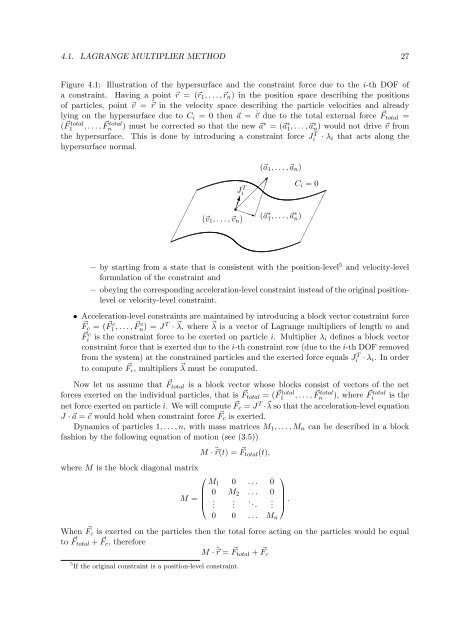
4.1. LAGRANGE MULTIPLIER METHOD 27 Figure 4.1: Illustration of the hypersurface and the constraint force due to the i-th DOF of a constraint. Having a point r = (r1, . . . , rn) in the position space describing the positions of particles, point v = ˙ r in the velocity space describing the particle velocities and already lying on the hypersurface due to Ci = 0 then a = ˙ v due to the total external force Ftotal = ( F total 1 , . . . , F total n ) must be corrected so that the new a ∗ = (a ∗ 1 , . . . ,a∗ n) would not drive v from the hypersurface. This is done by introducing a constraint force J T i · λi that acts along the hypersurface normal. ✁ ✁✁✁✁✁✁ (a1, . . . ,an) Ci = 0 ✂ ✂✍ J T i (v1, . . . , vn) ✒ (a ∗ 1 , . . . ,a∗ ✂ n) ✂✂✂✂ ✁ ✁✁✁✁✁✁ – by starting from a state that is consistent with the position-level 5 and velocity-level formulation of the constraint and – obeying the corresponding acceleration-level constraint instead of the original positionlevel or velocity-level constraint. • Acceleration-level constraints are maintained by introducing a block vector constraint force Fc = ( F c 1 , . . . , F c n) = J T · λ, where λ is a vector of Lagrange multipliers of length m and F c i is the constraint force to be exerted on particle i. Multiplier λi defines a block vector constraint force that is exerted due to the i-th constraint row (due to the i-th DOF removed from the system) at the constrained particles and the exerted force equals J T i · λi. In order to compute Fc, multipliers λ must be computed. Now let us assume that Ftotal is a block vector whose blocks consist of vectors of the net forces exerted on the individual particles, that is Ftotal = ( F total 1 , . . . , F total n ), where F total i is the net force exerted on particle i. We will compute Fc = J T · λ so that the acceleration-level equation J · a = c would hold when constraint force Fc is exerted. Dynamics of particles 1, . . . , n, with mass matrices M1, . . . , Mn can be described in a block fashion by the following equation of motion (see (3.5)) M · ¨ r(t) = Ftotal(t), where M is the block diagonal matrix ⎛ M1 ⎜ 0 M = ⎜ ⎝ . 0 M2 . . . . . . . . .. 0 0 . ⎞ ⎟ ⎠ 0 0 . . . Mn . When Fc is exerted on the particles then the total force acting on the particles would be equal to Ftotal + Fc, therefore M · ¨ r = Ftotal + Fc 5 If the original constraint is a position-level constraint.
Page 1: Univerzita Karlova v Praze Matemati
Page 5 and 6: Contents 1 Introduction 1 1.1 Backg
Page 7: CONTENTS vii 8 Figure Library 103 8
Page 10 and 11: x CONTENTS
Page 12 and 13: 2 CHAPTER 1. INTRODUCTION data from
Page 14 and 15: 4 CHAPTER 1. INTRODUCTION is capabl
Page 16 and 17: 6 CHAPTER 1. INTRODUCTION
Page 18 and 19: 8 CHAPTER 2. DIFFERENTIAL EQUATIONS
Page 20 and 21: 10 CHAPTER 2. DIFFERENTIAL EQUATION
Page 26 and 27: 16 CHAPTER 3. PARTICLE DYNAMICS dir
Page 28 and 29: 18 CHAPTER 3. PARTICLE DYNAMICS In
Page 30 and 31: 20 CHAPTER 3. PARTICLE DYNAMICS •
Page 32 and 33: 22 CHAPTER 3. PARTICLE DYNAMICS •
Page 34 and 35: 24 CHAPTER 4. CONSTRAINED PARTICLE
Page 46 and 47: 36 CHAPTER 5. RIGID BODY DYNAMICS D
Page 48 and 49: 38 CHAPTER 5. RIGID BODY DYNAMICS
Page 50 and 51: 40 CHAPTER 5. RIGID BODY DYNAMICS a
Page 52 and 53: 42 CHAPTER 5. RIGID BODY DYNAMICS v
Page 54 and 55: 44 CHAPTER 5. RIGID BODY DYNAMICS B
Page 56 and 57: 46 CHAPTER 5. RIGID BODY DYNAMICS S
Page 58 and 59: 48 CHAPTER 5. RIGID BODY DYNAMICS
Page 60 and 61: 50 CHAPTER 6. CONSTRAINED RIGID BOD
Page 86 and 87:
76 CHAPTER 6. CONSTRAINED RIGID BOD
Page 88 and 89:
Page 90 and 91:
Page 92 and 93:
Page 94 and 95:
Page 96 and 97:
Page 98 and 99:
Page 100 and 101:
90 CHAPTER 7. SIMULATOR on each oth
Page 102 and 103:
92 CHAPTER 7. SIMULATOR To run the
Page 104 and 105:
94 CHAPTER 7. SIMULATOR 7.3.3 Diffe
Page 106 and 107:
96 CHAPTER 7. SIMULATOR Simulation
Page 108 and 109:
98 CHAPTER 7. SIMULATOR depend on t
Page 110 and 111:
100 CHAPTER 7. SIMULATOR functions
Page 112 and 113:
102 CHAPTER 7. SIMULATOR Analogousl
Page 114 and 115:
104 CHAPTER 8. FIGURE LIBRARY Skele
Page 116 and 117:
106 CHAPTER 8. FIGURE LIBRARY The i
Page 118 and 119:
108 CHAPTER 8. FIGURE LIBRARY subtl
Page 120 and 121:
110 CHAPTER 9. RESULTS in the reduc
Page 122 and 123:
112 CHAPTER 9. RESULTS desks and no
Page 124 and 125:
114 CHAPTER 9. RESULTS Figure 9.2:
Page 126 and 127:
116 CHAPTER 9. RESULTS The produced
Page 128 and 129:
118 CHAPTER 9. RESULTS of optical m
Page 130 and 131:
120 CHAPTER 10. CONCLUSIONS The col
Page 132:
122 BIBLIOGRAPHY [16] Katsuaki Kawa
show all

thesis - Computer Graphics Group - Charles University - Univerzita ...

Create successful ePaper yourself

Delete template?

Save as template?