thesis - Computer Graphics Group - Charles University - Univerzita ...

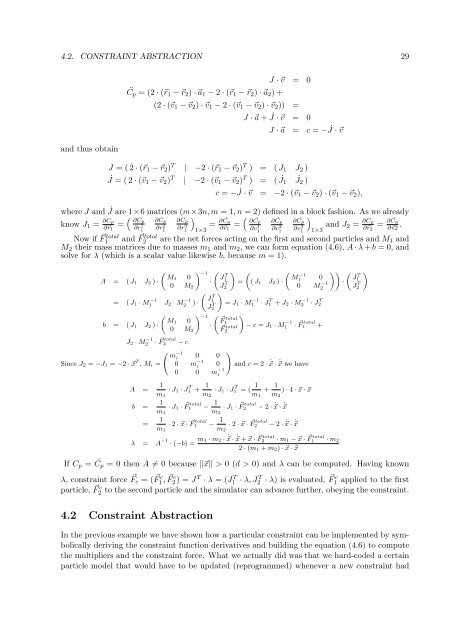
4.2. CONSTRAINT ABSTRACTION 29
and thus obtain
¨Cp = (2 · (r1 − r2) · a1 − 2 · (r1 − r2) · a2) +
J · v = 0
(2 · (v1 − v2) · v1 − 2 · (v1 − v2) · v2)) =
J · a + ˙
J · v = 0
J · a = c = − ˙
J · v
J = ( 2 · (r1 − r2) T | −2 · (r1 − r2) T ) = ( J1 J2 )
J ˙ = ( 2 · (v1 − v2) T | −2 · (v1 − v2) T ) = ( ˙ J1
˙
J2 )
c = − ˙
J · v = −2 · (v1 − v2) · (v1 − v2),
where J and ˙ J are 1×6 matrices (m×3n, m = 1, n = 2) defined in a block fashion. As we already
∂Cp
know J1 = ∂Cp
∂r1 =
∂r 1 1
∂Cp
∂r 2 1
∂Cp
∂r 3 1
1×3
= ∂ ˙
Cp
∂v1 =
∂ ˙
Cp
∂v 1 1
∂ ˙
Cp
∂v 2 1
∂ ˙
Cp
∂v 3 1
1×3 and J2 = ∂Cp
∂r2
= ∂ ˙
Cp
∂v2 .
Now if F total
1 and F total
2 are the net forces acting on the first and second particles and M1 and
M2 their mass matrices due to masses m1 and m2, we can form equation (4.6), A · λ + b = 0, and
solve for λ (which is a scalar value likewise b, because m = 1).
−1
T
M1 0 J1 A = ( J1 J2 ) ·
·
0 M2 J T
−1
M1 0
= ( J1 J2 ) ·
2
0 M −1
T
J1 ·
2 J T
2
= ( J1 · M −1
1 J2 · M −1
T
J1 2 ) ·
J T
= J1 · M
2
−1
1 · J T 1 + J2 · M −1
2 · J T 2
−1
M1 0
b = ( J1 J2 ) ·
·
− c = J1 · M
0 M2
−1
1 · F total
1 +
J2 · M −1
2
Since J2 = −J1 = −2 · x T , Mi =
A =
b =
=
· F total
2
1
m1
1
m1
1
m1
− c
m −1
i 0 0
0 m −1
i
F total
1
F total
2
0
0 0 m −1
i
· J1 · J T 1 + 1
m2
· J1 · F total
1 − 1
and c = 2 · ˙ x · ˙ x we have
· J1 · J T 1 = ( 1
m2
· 2 · x · F total
1 − 1
m2
· J1 · F total
2
m1
· 2 · x · F total
2
+ 1
) · 4 · x · x
m2
− 2 · ˙ x · ˙ x
λ = A −1 · (−b) = m1 · m2 · ˙ x · ˙ x + x · F total
2
− 2 · ˙ x · ˙ x
2 · (m1 + m2) · x · x
· m1 − x · F total
1
If Cp = ˙
Cp = 0 then A = 0 because x > 0 (d > 0) and λ can be computed. Having known
λ, constraint force Fc = ( F c 1 , F c 2 ) = J T · λ = (J T 1 · λ, J T 2 · λ) is evaluated, F c 1 applied to the first
particle, F c 2 to the second particle and the simulator can advance further, obeying the constraint.
4.2 Constraint Abstraction
In the previous example we have shown how a particular constraint can be implemented by symbolically
deriving the constraint function derivatives and building the equation (4.6) to compute
the multipliers and the constraint force. What we actually did was that we hard-coded a certain
particle model that would have to be updated (reprogrammed) whenever a new constraint had
· m2