2 Financial Markets and Transformation Functions
2 Financial Markets and Transformation Functions
2 Financial Markets and Transformation Functions

Create successful ePaper yourself
Turn your PDF publications into a flip-book with our unique Google optimized e-Paper software.
Prof. Dr. Hans-Peter Burghof, University of Hohenheim, Bank Management<br />
2 <strong>Financial</strong> <strong>Markets</strong> <strong>and</strong> <strong>Transformation</strong> <strong>Functions</strong><br />
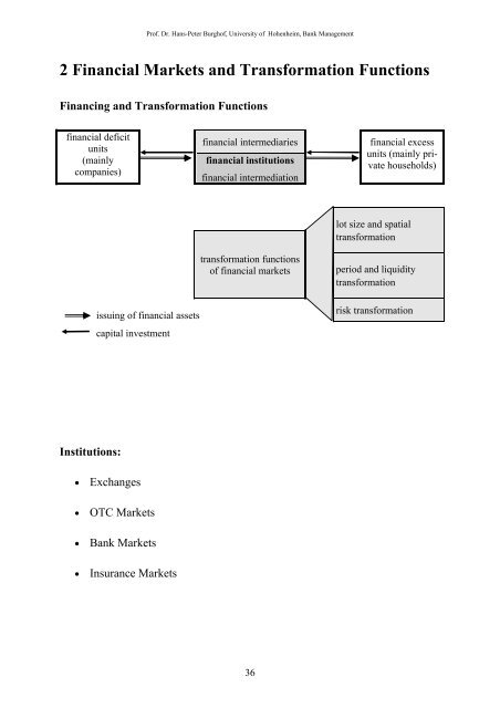
Financing <strong>and</strong> <strong>Transformation</strong> <strong>Functions</strong><br />
financial deficit<br />
units<br />
(mainly<br />
companies)<br />
Institutions:<br />
issuing of financial assets<br />
capital investment<br />
Exchanges<br />
OTC <strong>Markets</strong><br />
Bank <strong>Markets</strong><br />
Insurance <strong>Markets</strong><br />
financial intermediaries<br />
financial institutions<br />
financial intermediation<br />
transformation functions<br />
of financial markets<br />
36<br />
financial excess<br />
units (mainly private<br />
households)<br />
lot size <strong>and</strong> spatial<br />
transformation<br />
period <strong>and</strong> liquidity<br />
transformation<br />
risk transformation
Prof. Dr. Hans-Peter Burghof, University of Hohenheim, Bank Management<br />
a) Lot Size <strong>and</strong> Spatial <strong>Transformation</strong><br />
Spatial transformation:<br />
- Solvency at different places (monetary transactions, loans)<br />
- Capital transfers between regions financial balancing<br />
Effects of the failure of a banking system?<br />
Lot size transformation:<br />
- Matching investments of a different size<br />
- Pooling small deposits<br />
- Splitting large deposits<br />
37
Prof. Dr. Hans-Peter Burghof, University of Hohenheim, Bank Management<br />
b) Period <strong>and</strong> Liquidity <strong>Transformation</strong><br />
- Financing long-term investments with short-term funds (positive period<br />
transformation) <strong>and</strong> vice versa (negative period transformation)<br />
- Option to withdraw financial resources out of long-term projects prior to<br />
maturity<br />
Enabled by:<br />
Secondary markets<br />
Price <strong>and</strong> liquidity risks<br />
Possibility of hedging with particular financial products<br />
Intermediation<br />
Counter party risk for the investor<br />
Limited default risk of the financial intermediary by setting financing<br />
rules<br />
38
Prof. Dr. Hans-Peter Burghof, University of Hohenheim, Bank Management<br />
<strong>Financial</strong> Rules to Limit the Risks that Arise from Period <strong>and</strong> Liquidity Trans-<br />
formation<br />
Golden Banking Rule/Golden Rule of Finance:<br />
Total maturity matching<br />
Golden Rule of Balance Sheet<br />
Basis: “Schichtenbilanz”<br />
assets liabilities<br />
A1: Assets with a capital commitment of over<br />
4 years<br />
A2: Assets with a capital commitment of 3<br />
months to 4 years<br />
A3: Assets with a capital commitment up to 3<br />
months<br />
A1 ≤ F1 <strong>and</strong> A1+A2 ≤ F1+F2<br />
“Bodensatzregel” (Principles II <strong>and</strong> III of BAKred)<br />
Rule 1: A1 ≤ F1 + 0,6 F2 + 0,1 F3<br />
39<br />
F1: <strong>Financial</strong> resources invested longer than 4<br />
years<br />
F2: : <strong>Financial</strong> resources invested 3 months to<br />
4 years<br />
F3: : <strong>Financial</strong> resources invested less than 3<br />
months<br />
Rule 2: A2 ≤ (F1 + 0,6 F2 + 0,1 F3 - A1) + 0,4 F2 + 0,2 F3
c) Risk <strong>Transformation</strong><br />
Via secondary markets:<br />
Prof. Dr. Hans-Peter Burghof, University of Hohenheim, Bank Management<br />
Portfolio diversification: (stock) exchange or funds<br />
Limiting risk by using financial derivates<br />
Via financial intermediaries:<br />
Portfolio diversification <strong>and</strong> available net equity of a bank or insurance<br />
company<br />
Banks as “delegated monitor“ <strong>and</strong> “delegated contractor“<br />
Implementation by banks: Risk management<br />
40
Model Calculation<br />
Arrow-Debreu-Model:<br />
Prof. Dr. Hans-Peter Burghof, University of Hohenheim, Bank Management<br />
- 4 states with identical probability<br />
- 2 financial assets (A1 <strong>and</strong> A2)<br />
- Utility functions U or V<br />
- Amount of investment: 100<br />
state: s1 s2 s3 s4<br />
A1 x11 = 130 x12 = 130 x13 = 90 x14 = 90<br />
A2 x21 = 160 x22 = 60 x21 = 160 x22 = 60<br />
U <br />
x<br />
U(Al) 11,40 11,40 9,49 9,49<br />
U(A2) 12,65 7,75 12,65 7,75<br />
E(U(A1)) = 10,44 E(U(A2)) = 10,20<br />
<br />
V <br />
<br />
x<br />
x 5<br />
x 100<br />
otherwise<br />
V(A1) 11,40 11,40 4,49 4,49<br />
V(A2) 12,65 2,75 12,65 2,75<br />
E(V(A1)) = 7,94 E(V(A2)) = 7,70<br />
41
Prof. Dr. Hans-Peter Burghof, University of Hohenheim, Bank Management<br />
Risk <strong>Transformation</strong> by Diversification:<br />
state: s1 s2 s3 s4<br />
A1 x11 = 130 x12 = 130 x13 = 90 x14 = 90<br />
A2 x21 = 160 x22 = 60 x21 = 160 x22 = 60<br />
Portfolio formation: Purchase α = 50% of A1 <strong>and</strong> (1 – α) = 50% of A2<br />
½ A1 + ½ A2 xd1 = 145 xd2 = 95 xd3 = 125 xd4 = 75<br />
U(α = 50%) 12.04 9.75 11.18 8.66<br />
V(α = 50%) 12.04 4.75 11.18 3.66<br />
E(U(α = 50%)) = 10,40 E(V(α = 50%)) = 7,90<br />
(“naive” diversification, without success in this case)<br />
Portfolio formation:<br />
Purchase α = 86.52% of A1 <strong>and</strong> (1 - α) = 13.48% of A2<br />
xd1 = 134,04 xd2 = 120.56 xd3 = 99.44 xd4 = 85.96<br />
U(α = 86,52%) 11.58 10.98 9,97 9.27<br />
V(α = 86,52%) 11.58 10.98 4.97 4.27<br />
E(U(α = 86.52%)) = 10.45 E(V(α = 86.52%)) = 7.95<br />
(optimal diversification for utility function U)<br />
Instruments:<br />
Diversification via portfolio formation<br />
Buying shares in a fund<br />
Buying bank or insurance shares<br />
42
Prof. Dr. Hans-Peter Burghof, University of Hohenheim, Bank Management<br />
Risk <strong>Transformation</strong> by Risk Splitting:<br />
state: s1 s2 s3 s4<br />
A1 x11 = 130 x12 = 130 x13 = 90 x14 = 90<br />
A2 x21 = 160 x22 = 60 x21 = 160 x22 = 60<br />
“No-loss“ contract (e.g. on A1):<br />
xsl1 = 120 xsl2 = 120 xsl3 = 100 xsl4 = 100<br />
U(SL) = V(SL) 10,95 10,95 10 10<br />
Risk free asset:<br />
E(U(x)) = E(V(x)) = 10,47<br />
xrl1 = 110 xsl2 = 110 xsl3 = 110 xsl4 = 110<br />
U(RF) = V(RF) 10,49 10,49 10,49 10,49<br />
E(U(x)) = E(V(x)) = 10,49<br />
Hedging or financial engineering by:<br />
Contracting with a bank<br />
A particular fund construction<br />
Buying financial assets on the capital market<br />
43
Prof. Dr. Hans-Peter Burghof, University of Hohenheim, Bank Management<br />
<strong>Financial</strong> Engineering on the Capital Market:<br />
E.g.: Combination of shares in A1 <strong>and</strong> a (long) put option<br />
Wealth of the investor<br />
in T<br />
State: s1 s2 s3 s4<br />
A1 (α of 100) α130 α130 α90 α90<br />
Put option with<br />
strike P on α A1<br />
0 0 α(P – 90) α(P – 90)<br />
Desired cash flow xsl1 = 120 xsl2 = 120 xsl3 = 100 Xsl4 = 100<br />
130<br />
120 <br />
90<br />
<br />
Costs:<br />
Desired<br />
Minimum Wealth<br />
in T<br />
(e.g. 100)<br />
12<br />
13<br />
100<br />
<br />
100 13<br />
12<br />
P90100 P 108,<br />
3<br />
(risk free interest rate i = 10% <strong>and</strong> risk neutral valuation of the option)<br />
Buying shares of the asset A1:<br />
Buying a put option 1<br />
<br />
on share α of the asset : 2<br />
Total costs :<br />
Portfolio<br />
A1<br />
1 1 12<br />
108, 3 90<br />
108, 3 90<br />
92,<br />
31<br />
Put Option<br />
<br />
7,<br />
69<br />
100<br />
<br />
100<br />
44<br />
1<br />
i<br />
92,<br />
31<br />
Value of the Asset in T<br />
2 13<br />
1<br />
1,<br />
1<br />
<br />
7,<br />
69