The Hartree-Fock approximation underlies the most commonly used ...
The Hartree-Fock approximation underlies the most commonly used ...
The Hartree-Fock approximation underlies the most commonly used ...

Create successful ePaper yourself
Turn your PDF publications into a flip-book with our unique Google optimized e-Paper software.
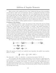
IIb. <strong>The</strong> <strong>Hartree</strong>-<strong>Fock</strong> Approximation:<br />
<strong>The</strong> <strong>Hartree</strong>-<strong>Fock</strong> <strong>approximation</strong> <strong>underlies</strong> <strong>the</strong> <strong>most</strong> <strong>commonly</strong> <strong>used</strong> method in chemistry<br />
for calculating electron wave functions of atoms and molecules. It is <strong>the</strong> best <strong>approximation</strong><br />
to <strong>the</strong> true wave function where each electron is occupying an orbital, <strong>the</strong> picture<br />
that <strong>most</strong> chemists use to rationalize chemistry. <strong>The</strong> <strong>Hartree</strong>-<strong>Fock</strong> <strong>approximation</strong> is, fur<strong>the</strong>rmore,<br />
<strong>the</strong> usual starting point for more accurate calculations that can, in principle,<br />
become exact.<br />
It is <strong>most</strong> convenient to use ’atomic units’ in calculations of electronic wave functions<br />
for atoms and molecules. <strong>The</strong> unit chosen for<br />
length is <strong>the</strong> Bohr radius a0,<br />
mass is <strong>the</strong> electron mass me,<br />
charge is <strong>the</strong> electron charge e,<br />
energy is <strong>the</strong> <strong>Hartree</strong> = 27.211 eV = 2 EI,<br />
where EI is <strong>the</strong> energy of <strong>the</strong> ground state of <strong>the</strong> hydrogen atom with respect to separated<br />
electron and proton. In <strong>the</strong>se units, ¯h becomes unity.<br />
<strong>The</strong> full Hamiltonian for a system of N electrons in <strong>the</strong> presence of M nuclei with<br />
charge ZA <strong>the</strong>n becomes<br />
where<br />
H exact =<br />
N<br />
i<br />
h(i) +<br />
h(i) ≡ − 1<br />
2 ∇2 i −<br />
and riA is <strong>the</strong> distance between nucleus A and electron i.<br />
Solving <strong>the</strong> Schrödinger equation with this Hamiltonian is very difficult because <strong>the</strong><br />
1/rij terms correlate <strong>the</strong> distribution of all <strong>the</strong> electrons. As is frequently done with such<br />
many body problems, we will seek a mean field <strong>approximation</strong>, where each electron is<br />
treated separately and <strong>the</strong> effect of all <strong>the</strong> o<strong>the</strong>r electrons is included in an average way.<br />
<strong>The</strong> way this is done is to carry out a variational calculation where <strong>the</strong> trial function is of<br />
<strong>the</strong> form of a single Slater determinant<br />
That is, <strong>the</strong> expectation value of <strong>the</strong> energy<br />
N<br />
i<br />
M<br />
A<br />
N<br />
j>i<br />
ZA<br />
riA<br />
|ψ0 >= |χ1χ2 . . .χN > .<br />
.<br />
1<br />
rij<br />
E0 = < H > = < ψ0|H|ψ0 ><br />
is minimized with respect to <strong>the</strong> determinantal trial function |ψ0 >. In <strong>the</strong> process an<br />
optimal single determinant <strong>approximation</strong> to <strong>the</strong> stationary state wave function is obtained.<br />
Such a form of <strong>the</strong> function can, however, only be exact if <strong>the</strong> Hamiltonian separates into<br />
terms where each one only depend on one of <strong>the</strong> electron coordinates. Since <strong>the</strong> true<br />
32
Hamiltonian does contain terms of <strong>the</strong> form 1/rij, this procedure can never yield an exact<br />
solution. But, it is a useful first <strong>approximation</strong>.<br />
One can better understand <strong>the</strong> <strong>approximation</strong> being made here by thinking of <strong>the</strong><br />
resulting eigen function as an exact solution to a different problem, one where <strong>the</strong> Hamiltonian<br />
is an <strong>approximation</strong> to <strong>the</strong> true Hamiltonian<br />
H app =<br />
N<br />
i<br />
<br />
h(i)+v HF<br />
<br />
i (i) = H1 + H2 + . . .HN.<br />
Here, v HF<br />
i (i) is an effective potential experienced by <strong>the</strong> i−th electron due to <strong>the</strong> presence<br />
of <strong>the</strong> o<strong>the</strong>r electrons, but it cannot depend on <strong>the</strong> coordinates of <strong>the</strong> o<strong>the</strong>r electrons and<br />
thus represents a spatially averaged interaction. During <strong>the</strong> variational optimization of <strong>the</strong><br />
spin-orbitals an optimal effective interaction v HF<br />
i (i) is obtained as well as <strong>the</strong> stationary<br />
state wave functions. Since <strong>the</strong> approximate Hamiltonian H app separates, its eigenfunctions<br />
can indeed be written as a Slater determinant formed from spin-orbitals<br />
|ψ0 >= |χ1χ2 . . .χN > .<br />
<strong>The</strong> variational minimization of <strong>the</strong> energy with respect to arbitrary variations of <strong>the</strong><br />
spin-orbitals leads to equations for <strong>the</strong> spin-orbitals and <strong>the</strong> optimal, effective potential.<br />
<strong>The</strong> derivation of <strong>the</strong>se equations, called <strong>the</strong> <strong>Hartree</strong>-<strong>Fock</strong> equations is given below. <strong>The</strong><br />
expectation value of <strong>the</strong> Hamiltonian for a Slater determinant wave function was previously<br />
found to be<br />
N<br />
E0 = [a|h|a] + 1<br />
N N<br />
[aa|bb] − [ab|ba]<br />
2<br />
a<br />
where <strong>the</strong> summation indices a and b range over all occupied spin-orbitals. In searching<br />
for <strong>the</strong> optimal wave function, we must impose <strong>the</strong> constraint that all <strong>the</strong> spin-orbitals<br />
remain orthonormal, i.e.<br />
[a|b] − δab = 0<br />
for a = 1, 2, . . ., N and b = 1, 2, . . ., N, a total of N 2 constraints.<br />
<strong>The</strong> standard method for finding an extremum (minimum or maximum) subject to<br />
a constraint is Lagrange’s method of undetermined multipliers: <strong>The</strong> constraint equations<br />
are each multiplied by some constant and added to <strong>the</strong> expression to be optimized. Thus,<br />
we define a new functional L:<br />
L ≡ E0 −<br />
N<br />
a<br />
N<br />
b<br />
a<br />
ǫba<br />
b<br />
<br />
[a|b] − δab .<br />
When <strong>the</strong> constraints are satisfied, this new quantity equals <strong>the</strong> expectation value of <strong>the</strong><br />
Hamiltonian, E0. <strong>The</strong> unknown constants ǫba are <strong>the</strong> Lagrange multipliers. <strong>The</strong> quantity<br />
L (as well as E0) is a functional of <strong>the</strong> spin-orbitals χa, χb, . . ., χN and <strong>the</strong> problem is<br />
33
to find stationary points of L. That is, given infinitesimal change in <strong>the</strong> spin-orbitals,<br />
χa → χa + δχa, <strong>the</strong> change in L, (L → L + δL), should be zero, i.e.:<br />
0 = δL = δE0 −<br />
N<br />
a=1<br />
N<br />
b=1<br />
ǫba δ[a|b] .<br />
We now evaluate <strong>the</strong> terms on <strong>the</strong> right hand side of this expression. By inserting <strong>the</strong><br />
new spin-orbitals χa + δχa, etc. into <strong>the</strong> expression for E0, and using <strong>the</strong> fact that <strong>the</strong><br />
integration indicated by [ ] is a linear operation, <strong>the</strong> change in E0 is to first order:<br />
δE0 =<br />
+ 1<br />
2<br />
N<br />
a=1<br />
([δχa|h|χa] + [χa|h|δχa])<br />
N<br />
a=1<br />
N<br />
b=1<br />
<br />
[δχaχa|χbχb] + [χaδχa|χbχb] + [χaχa|δχbχb] + [χaχa|χbδχb]<br />
<br />
− [δχaχb|χbχa] − [χaδχb|χbχa] − [χaχb|δχbχa] − [χaχb|χbδχa] .<br />
From <strong>the</strong> definition of <strong>the</strong> integrals it is clear that [δχa|h|χa] ∗ = [χa|h|δχa] and [δχaχa|χbχb] ∗ =<br />
[χaδχa|χbχb], etc. Fur<strong>the</strong>rmore, [δχaχa|χbχb] = [χbχb|δχaχa] as can be seen by relabeling<br />
<strong>the</strong> integration variables representing <strong>the</strong> electron coordinates. <strong>The</strong> change in E0 can<br />
<strong>the</strong>refore be rewritten as:<br />
δE0 =<br />
N<br />
[δχa|h|χa] +<br />
a=1<br />
N<br />
a=1<br />
N<br />
[δχaχa|χbχb] − [δχaχb|χbχa] + c.c.<br />
b=1<br />
<strong>The</strong> notation c.c. stands for complex conjugate.<br />
Using <strong>the</strong> factor rule of differentiation on <strong>the</strong> second term in <strong>the</strong> expression for δL<br />
gives<br />
ab<br />
δ[a|b] = δ[χa|χb] = [δχa|χb] + [χa|δχb]<br />
<br />
ǫbaδ[χa|χb] = <br />
ǫba[δχa|χb] + <br />
ǫba[χa|δχb] .<br />
ab<br />
Interchanging <strong>the</strong> summation indices a and b in <strong>the</strong> second sum on <strong>the</strong> right hand side<br />
gives: <br />
ǫbaδ[χa|χb] = <br />
ǫba[δχa|χb] + <br />
ǫab[χb|δχa] .<br />
ab<br />
ab<br />
L is a real quantity and by taking <strong>the</strong> complex conjugate of <strong>the</strong> expression defining L, it<br />
can be shown that ǫba = ǫ∗ ab , that is <strong>the</strong> Lagrange multipliers are elements of a Hermitian<br />
matrix. This means <strong>the</strong> second sum is just <strong>the</strong> complex conjugate of <strong>the</strong> first, and we have<br />
<br />
ab<br />
ǫbaδ[χa|χb] = <br />
ab<br />
34<br />
ab<br />
ab<br />
ǫba[δχa|χb] + c.c..
Finally, <strong>the</strong> expression for δL becomes:<br />
δL =<br />
N<br />
[δχa|h|χa] +<br />
a=1<br />
N<br />
a=1<br />
N<br />
b=1<br />
<br />
<br />
[δχaχa|χbχb] − [δχaχb|χbχa] − ǫba[δχa|χb] + c.c.<br />
In this expression we have [δχa appearing on <strong>the</strong> left hand side of each term. We can<br />
symbolically rewrite<br />
δL =<br />
N<br />
[δχa<br />
a=1<br />
<br />
|h|χa] +<br />
N<br />
<br />
{χa|χbχb] − χb|χbχa] − ǫba|χb]} + c.c.<br />
b=1<br />
More explicitly, <strong>the</strong> expresssion for δL is<br />
δL =<br />
N<br />
<br />
a=1<br />
dx1δχ ∗ a<br />
<br />
h(1)χa(1) +<br />
N<br />
{ Jb(1) − Kb(1) <br />
χa(1) − ǫbaχb(1)} + c.c.<br />
b=1<br />
where we have defined two new operators, J and K. <strong>The</strong> Coulomb operator, Jb, is defined<br />
as<br />
<br />
2 1<br />
Jb(1) ≡ dx2 |χb(2)|<br />
r12<br />
such that<br />
and, in particular we have<br />
<br />
Jb(1)χa(1) =<br />
<br />
dx2χ ∗ b(2) 1<br />
r12<br />
<br />
χb(2) χa(1)<br />
dx1 χ ∗ a(1)Jb(1)χa(1) = [aa|bb] .<br />
<strong>The</strong> exchange operator, Kb(1), is defined such that<br />
<br />
Kb(1)χa(1) ≡ dx2χ ∗ b(2) 1<br />
r12<br />
<br />
χa(2) χb(1) .<br />
Note how <strong>the</strong> labels a and b on spin-orbitals for electron 1 get interchanged. In particular,<br />
we have <br />
dx1 χ ∗ a (1)Kb(1)χa(1) = [ab|ba] .<br />
Note that <strong>the</strong> exchange operator is a non-local operator in that <strong>the</strong>re does not exist<br />
a simple potential function giving <strong>the</strong> action of <strong>the</strong> operator at a point x1. <strong>The</strong> result of<br />
operating with Kb(1) on χa(1) depends on χa throughout all space (not just at x1).<br />
Now set δL = 0 to obtain <strong>the</strong> optimal spin-orbitals. Since δχ∗ a is arbitrary, we must<br />
have <br />
N<br />
<br />
N<br />
h(1) + {Jb(1) − Kb(1)} χa(1) = ǫbaχb(1)<br />
b=1<br />
35<br />
b=1
for each spin-orbital χa with a = 1, 2, . . ., N. Defining <strong>the</strong> <strong>Fock</strong> operator as<br />
f(1) ≡ h(1) +<br />
N<br />
{Jb(1) − Kb(1)} ,<br />
<strong>the</strong> solution to <strong>the</strong> optimization problem, i.e. <strong>the</strong> optimal spin-orbitals, satisfy<br />
f χa =<br />
b<br />
N<br />
b=1<br />
ǫba χb .<br />
This equation can be diagonalized, i.e., we can find a unitary transformation of <strong>the</strong><br />
spin-orbitals that diagonalizes <strong>the</strong> matrix ǫ which has matrix elements ǫba. <strong>The</strong> <strong>Fock</strong><br />
operator is invariant under a unitary transformation, that is a transformation where a new<br />
set of spin-orbitals is defined by taking a linear combinations. <strong>The</strong> new set of spin-orbitals<br />
is defined as<br />
χ ′ a = <br />
b<br />
χbUba<br />
where U † = U −1 such that ˜ǫ ′ = U † ˜ǫ U is diagonal. <strong>The</strong>n<br />
f χ ′ a = ǫ ′ a χ ′ a .<br />
This is <strong>the</strong> <strong>Hartree</strong>-<strong>Fock</strong> equation, a one electron equation for <strong>the</strong> optimal spin-orbitals. It<br />
is non-linear, since <strong>the</strong> <strong>Fock</strong> operator, f, itself depends on <strong>the</strong> spin-orbitals χa.<br />
Occupied and Virtual Orbitals:<br />
From <strong>the</strong> <strong>Hartree</strong>-<strong>Fock</strong> equation we get a set of spin-orbitals (dropping <strong>the</strong> primes<br />
now):<br />
fχj = ǫjχj j = 1, 2, . . ., ∞.<br />
By solving this equation we can generate an infinit number of spin-orbitals. <strong>The</strong> <strong>Fock</strong> operator,<br />
f, depends on <strong>the</strong> N spin-orbitals that have electrons, <strong>the</strong> occupied orbitals. Those<br />
will be labeled with a, b, c, .... Once <strong>the</strong> occupied orbitals have been found, <strong>the</strong> <strong>Hartree</strong>-<br />
<strong>Fock</strong> equation becomes an ordinary, linear eigenvalue equation and an infinit number of<br />
spin-orbitals with higher energies can be generated. Those are called virtual orbitals and<br />
will be labeled with r, s, ....<br />
<strong>The</strong> orbital energy<br />
What is <strong>the</strong> significance of <strong>the</strong> orbital energies ǫi? Left multiplying <strong>the</strong> <strong>Hartree</strong>-<strong>Fock</strong><br />
equation with < χi| gives<br />
< χi|f|χj >= ǫi < χi|χj >= ǫjδij .<br />
36
<strong>The</strong>refore<br />
ǫi = [χi|f|χi]<br />
N<br />
= [χi|h + (Jb − Kb)|χi]<br />
b<br />
= [i|h|i] + <br />
[ii|bb] − [ib|bi]<br />
b<br />
where <strong>the</strong> summation index, b, runs over all occupied spin-orbitals.<br />
<strong>The</strong> first term < i|h|i > is a one body energy, <strong>the</strong> electron kinetic energy and <strong>the</strong><br />
attractive interaction with <strong>the</strong> fixed nuclei. <strong>The</strong> second term, <strong>the</strong> sum over all occupied<br />
spin-orbitals, is a sum of two body interactions, <strong>the</strong> Coulomb and exchange interaction<br />
between electron i and <strong>the</strong> electrons in all occupied spin-orbitals. <strong>The</strong> total energy of <strong>the</strong><br />
system is not just <strong>the</strong> sum of ǫi for all occupied orbitals, because <strong>the</strong>n <strong>the</strong> pairwise terms<br />
would be double counted. Recall <strong>the</strong> expression for E0:<br />
E0 =<br />
N<br />
a<br />
[a|h|a] + 1<br />
2<br />
N<br />
a<br />
N<br />
[aa|bb] − [ab|ba] = <br />
b<br />
<strong>The</strong> factor 1/2 prevents double counting <strong>the</strong> two electron integrals.<br />
<strong>The</strong> significance of <strong>the</strong> ǫi becomes apparent when we add or subtract an electron to<br />
<strong>the</strong> N electron system. If we assume <strong>the</strong> spin-orbitals do not change when we, for example,<br />
remove an electron from spin-orbital χc, <strong>the</strong>n <strong>the</strong> determinant describing <strong>the</strong> N −1 electron<br />
system is<br />
| N−1 ψc >= |χ1χ2 . . .χc−1χc+1 . . .χN ><br />
with energy<br />
N−1<br />
Ec =< N−1 ψc|H|ψ N−1<br />
c<br />
= <br />
a=c<br />
[a|h|a] + 1<br />
2<br />
><br />
<br />
[aa|bb] − [ab|ba].<br />
<strong>The</strong> energy required to remove <strong>the</strong> electron, which is called <strong>the</strong> ionization potential, is:<br />
a=c<br />
b=c<br />
IP = N−1 Ec − E0<br />
= −[c|h|c] − 1<br />
N [cc|bb] − [cb|bc] +<br />
2<br />
b<br />
N<br />
a<br />
a<br />
ǫa .<br />
<br />
[aa|cc] − [ac|ca] .<br />
We do not need to restrict <strong>the</strong> summation to exclude c since <strong>the</strong> [cc|cc] term cancels out.<br />
Using <strong>the</strong> fact that [ac|ac] = [ca|ca] this can be rewritten as<br />
IP = −[c|h|c] −<br />
= −ǫc .<br />
N<br />
[cc|bb] − [cb|bc]<br />
b<br />
37
So, <strong>the</strong> orbital energy is simply <strong>the</strong> ionization energy.<br />
Similarly, after adding an electron to <strong>the</strong> N-electron system into a virtual orbital χr,<br />
<strong>the</strong> state is<br />
| N+1 ψr >= |χ1χ2 . . .χNχr ><br />
and <strong>the</strong> energy is<br />
N+1 Er = < N+1 ψr|H|ψ N+1<br />
r<br />
<strong>The</strong> energy difference is called <strong>the</strong> electron affinity, EA. Assuming <strong>the</strong> spin-orbitals stay<br />
<strong>the</strong> same, we have<br />
EA = E0 − N+1 Er = − ǫr.<br />
Koopman’s Rule:<br />
<strong>The</strong> orbital energy ǫi is <strong>the</strong> ionization potential for removing an electron from an<br />
occupied orbital χi or <strong>the</strong> electron affinity for adding an electron into virtual orbital χi,<br />
in ei<strong>the</strong>r case assuming <strong>the</strong> spin-orbitals do not change when <strong>the</strong> number of electrons is<br />
changed. This is a remarkably good <strong>approximation</strong> due apparently to cancellations of<br />
corrections due to adjustments in <strong>the</strong> orbitals.<br />
Restricted <strong>Hartree</strong>-<strong>Fock</strong>:<br />
For computational purposes, we would like to integrate out <strong>the</strong> spin functions α and β.<br />
This is particularly simple when we have spatial orbitals that are independent of spin, in<br />
<strong>the</strong> sense that a given spatial orbital can be <strong>used</strong> twice, once for spin up and once for spin<br />
down. For example, from a spatial orbital ψa we can generate two orthogonal spin-orbitals<br />
χ1 and χ2:<br />
χ1(x) = ψa(r)α(ω)<br />
χ2(x) = ψa(r)β(ω) .<br />
Determinants constructed from such spin-orbitals are called restricted determinants.<br />
Transition from Spin Orbitals to Spatial Orbitals:<br />
<strong>The</strong> restricted determinant can be written as<br />
|ψ > = |χ1χ2χ3 . . .χN−1χN ><br />
> .<br />
= |ψ1 ¯ ψ1ψ2 ¯ ψ2 . . .ψ N/2 ¯ ψN/2 ><br />
where <strong>the</strong> ψi denote spatial orbitals occupied by a spin-up electron and ¯ ψi denote <strong>the</strong> same<br />
spatial orbitals occupied by a spin-down electron.<br />
<strong>The</strong> energy of a determinantal wave function is<br />
E =< ψ|H|ψ >=<br />
N<br />
a<br />
[a|h|a] + 1<br />
2<br />
38<br />
N<br />
a<br />
N<br />
[aa|bb] − [ab|ba].<br />
b
We will, fur<strong>the</strong>rmore, assume here that all <strong>the</strong> electrons are paired (closed shell). <strong>The</strong><br />
wave function <strong>the</strong>n contains N/2 spin orbitals with spin up and N/2 spin orbitals with<br />
spin down, and we can write:<br />
N<br />
a<br />
χa =<br />
N/2<br />
<br />
a<br />
(ψa + ¯ ψa ).<br />
Any one electron integral involving spin-orbitals with opposite spin vanishes because of<br />
<strong>the</strong> orthogonality of <strong>the</strong> spin functions, α ∗ β dω = 0. For example,<br />
[ψi|h| ¯ ψj] = [ ¯ ψi|h|ψj] = 0 .<br />
Since <strong>the</strong> spin functions are normalized, |α| 2 dw = 1, <strong>the</strong> integration over spin does not<br />
affect <strong>the</strong> value of non-vanishing matrix elements. We <strong>the</strong>refore define yet ano<strong>the</strong>r notation<br />
for matrix elements<br />
(ψi|h|ψj) ≡ [ψi|h|ψj] = [ ¯ ψi|h| ¯ ψj].<br />
<strong>The</strong> round brackets indicate spatial integration only. Spin has already been integrated out.<br />
Similarly, for two electron integrals:<br />
[ψiψj|ψkψℓ] = [ψiψj| ¯ ψk ¯ ψℓ]<br />
= [ ¯ ψi ¯ ψj|ψkψℓ]<br />
= [ ¯ ψi ¯ ψj| ¯ ψk ¯ ψℓ]<br />
≡ (ψiψj|ψkψℓ).<br />
Any two electron integral with only one bar on ei<strong>the</strong>r side vanishes, for example:<br />
[ψi ¯ ψj|ψkψl] = [ψ ¯ ψj|ψk ¯ ψl] = 0.<br />
<strong>The</strong> energy for a single determinant wave function becomes:<br />
N/2 <br />
E = 2<br />
+<br />
a<br />
N/2<br />
<br />
a<br />
a<br />
(ψa|h|ψa)<br />
N/2<br />
<br />
b<br />
2(ψaψa|ψbψb) − (ψaψb|ψbψa)<br />
= 2 <br />
(a|h|a) + <br />
2(aa|bb) − (ab|ba)<br />
ab<br />
with <strong>the</strong> summation being over <strong>the</strong> spatial orbitals only. <strong>The</strong> first type of two electron<br />
integrals, Jij ≡ (ii|jj), is called <strong>the</strong> Coulomb integral since it represents <strong>the</strong> classical<br />
Coulomb repulsion between <strong>the</strong> charge clouds |ψi(r)| 2 and |ψj(r)| 2 . <strong>The</strong> second type,<br />
Kij ≡ (ij|ji), is called exchange integral and does not have a classical interpretation but<br />
39
arises from <strong>the</strong> antisymmetrization of <strong>the</strong> wave function. It results from <strong>the</strong> exchange<br />
correlation. <strong>The</strong> energy of two electrons in orbitals ψ1 and ψ2 is<br />
if <strong>the</strong>ir spin is antiparallel, but<br />
E(↑↓) = h11 + h22 + J12<br />
E(↑↑) = h11 + h22 + J12 − K12<br />
if <strong>the</strong>ir spin is parallel. <strong>The</strong> energy is lower when <strong>the</strong> spin is parallel (K12 > 0) because<br />
<strong>the</strong> antisymmetrization prevents <strong>the</strong> electrons from being at <strong>the</strong> same location.<br />
In summary: Given a determinantal wave function, <strong>the</strong> energy can be obtained in<br />
<strong>the</strong> following way:<br />
(1) each electron in spatial orbital ψi contributes hii to <strong>the</strong> energy,<br />
(2) each unique pair of electrons contributes Jij (irrespective of spin),<br />
(3) each pair of electons with parallel spin contributes −Kij.<br />
Restricted <strong>Hartree</strong>-<strong>Fock</strong> equation<br />
Using <strong>the</strong> above expression for <strong>the</strong> energy, <strong>the</strong> <strong>Hartree</strong>-<strong>Fock</strong> equation becomes:<br />
f(1)ψj(1) = ǫjψj(1)<br />
where <strong>the</strong> <strong>Fock</strong> operator can now be expressed as:<br />
f(1) = h(1) +<br />
N/2<br />
<br />
a<br />
2Ja(1) − Ka(1)<br />
and <strong>the</strong> restricted Coulomb and exchange operators are:<br />
<br />
Ja(1) = dr2ψ ∗ a(r2) 1<br />
ψa(r2)<br />
and<br />
<br />
Ka(1)ψi(1) =<br />
<br />
r12<br />
dr2ψ ∗ 1<br />
a (r2)<br />
r12<br />
<strong>The</strong> total energy of <strong>the</strong> system can be written as:<br />
N/2 <br />
E = 2<br />
a<br />
N/2 <br />
= 2<br />
a<br />
(a|h|a) +<br />
haa + <br />
a<br />
N/2<br />
<br />
a<br />
<br />
b<br />
40<br />
N/2<br />
<br />
b<br />
<br />
ψi(r2) ψa(r1) .<br />
2(aa|bb) − (ab|ba)<br />
2Jab − Kab
and <strong>the</strong> orbital energies are:<br />
ǫi = (i|h|i) +<br />
N/2<br />
<br />
b<br />
2(ii|bb) − (ib|bi) = hii +<br />
N/2<br />
<br />
b<br />
2Jib − Kib<br />
All <strong>the</strong>se expresssions are in terms of <strong>the</strong> spatial orbitals only, <strong>the</strong>re is no explicit reference<br />
to spin.<br />
<strong>The</strong> Roothaan Equations:<br />
<strong>The</strong> spatial <strong>Hartree</strong>-<strong>Fock</strong> equation:<br />
f(r1)ψi(r1) = ǫi ψi(r1)<br />
can be solved numerically for atoms. <strong>The</strong> results of such calculations have been tabulated<br />
by Hermann and Skilman. However, for molecules <strong>the</strong>re is no practical procedure known<br />
for solving <strong>the</strong> equation directly (recall f depends on <strong>the</strong> orbitals) and <strong>the</strong> orbitals ψi are<br />
instead expanded in some known basis functions φµ:<br />
ψi =<br />
K<br />
µ<br />
Cµi φµ<br />
i = 1, 2, . . ., K.<br />
If <strong>the</strong> number of basis functions is K, we can generate K different orbitals. If <strong>the</strong> set {φµ}<br />
is complete <strong>the</strong> results would be <strong>the</strong> same as a direct numerical solution to <strong>the</strong> <strong>Hartree</strong>-<br />
<strong>Fock</strong> equation. But, for practical reasons <strong>the</strong> set {φµ} is always finite and <strong>the</strong>refore not<br />
complete and some error is introduced by expanding ψi. This is called <strong>the</strong> basis set error.<br />
<strong>The</strong> problem now is reduced to determining <strong>the</strong> expansion coefficients Cµi. Inserting<br />
<strong>the</strong> expansion into <strong>the</strong> <strong>Hartree</strong>-<strong>Fock</strong> equation gives<br />
f(1) <br />
γ<br />
Cγiφγ(1) = ǫi<br />
Left multiplying with φ∗ µ (1) and integrating gives:<br />
<br />
γ<br />
Cγi<br />
<br />
<br />
dr1φ ∗ <br />
µ(1)f(1)φγ(1) = ǫi<br />
<br />
≡ Fµγ<br />
<strong>the</strong> <strong>Fock</strong> matrix<br />
γ<br />
<br />
γ<br />
FµγCγi = ǫi<br />
<br />
γ<br />
˜F ˜ C = ˜ S ˜ C¯ǫ.<br />
41<br />
γ<br />
Cγiφγ(1).<br />
Cγi<br />
SµγCγi<br />
<br />
dr1φ ∗ µ(1)φγ(1)<br />
<br />
≡ Sµγ<br />
<br />
<strong>the</strong> overlap matrix
This is a matrix representation of <strong>the</strong> <strong>Hartree</strong>-<strong>Fock</strong> equation and is called <strong>the</strong> Roothaan<br />
equations. <strong>The</strong> matrices ˜ F, ˜ S and ˜ C are K × K matrices and ¯ǫ is a vector of length K.<br />
<strong>The</strong> problem is <strong>the</strong>refore reduced to solving algebraic equations using matrix techniques.<br />
Only if K → ∞ are <strong>the</strong> Roothan equations equivalent to <strong>the</strong> <strong>Hartree</strong>-<strong>Fock</strong> equation.<br />
<strong>The</strong> Roothaan equations are non-linear:<br />
˜F ( ˜ C) ˜ C = ˜ S ˜ C¯ǫ.<br />
Since ˜ F depends on ˜ C and <strong>the</strong>refore <strong>the</strong>y need to be solved in an iterative fashion. Given<br />
an estimate for ˜ Cn we can find an estimate for ˜ F ( Cn) ˜ and <strong>the</strong>n solve <strong>the</strong> equation<br />
˜F ( ˜Cn) ˜ Cn+1 = ˜ S ˜ Cn+1¯ǫ<br />
to obtain a new estimate for <strong>the</strong> ˜ C matrix. If ˜ Cn+1 = ˜ Cn to within reasonable tolerance<br />
<strong>the</strong>n self consistency has been achieved and ˜ Cn is <strong>the</strong> solution. Most workers refer to such<br />
a solution as self-consistent-field (SCF) solution for any finite basis set {φi} and reserve<br />
<strong>the</strong> term <strong>Hartree</strong>-<strong>Fock</strong> limit to <strong>the</strong> infinite basis solution. <strong>The</strong> equation is solved at each<br />
step by diagonalizing <strong>the</strong> overlap matrix ˜ S, i.e., by finding a unitary transformation ˜ X<br />
such that<br />
X † SX = 1.<br />
<strong>The</strong> transformed basis function are<br />
φ ′ µ = <br />
and form an orthonormal set, i.e.,<br />
γ<br />
<br />
Xγµφγ<br />
drφ ′∗ µ φ′ γ<br />
µ = 1, 2, . . ., K<br />
= δµγ.<br />
<strong>The</strong>n <strong>the</strong> equation becomes an ordinary eigenvalue equation:<br />
F ′ C ′ = C ′ ǫ where F ′ ≡ X † FX and C ′ ≡ X −1 C.<br />
<strong>The</strong> main computational effort in doing a large SCF calculation lies in <strong>the</strong> evaluation of<br />
<strong>the</strong> two-electron integrals. If <strong>the</strong>re are K basis functions <strong>the</strong>n <strong>the</strong>re will be on <strong>the</strong> order<br />
of K 4 /8 unique two-electron integrals. This can be on <strong>the</strong> order of millions even for small<br />
basis sets and moderately large molecules. <strong>The</strong> accuracy and efficiency of <strong>the</strong> calculation<br />
depends very much on <strong>the</strong> choice of basis functions, just as any variational calculation<br />
depends strongly on <strong>the</strong> choice of trial functions.<br />
Basis Set Functions:<br />
Two types of basis functions are frequently <strong>used</strong>:<br />
42
(1) Slater type functions, which for a 1S orbital centered at RA has <strong>the</strong> form<br />
with ζ a free parameter and<br />
(2) Gaussian type function<br />
with α a free parameter.<br />
φ SF<br />
1S (ζ,r − RA) = ζ/π e −ζ|r− RA|<br />
φ GF<br />
1S (α,r − RA) =<br />
3/2 2α<br />
π<br />
e −α|r− RA| 2<br />
<strong>The</strong> Slater type functions have a shape which matches better <strong>the</strong> shape of typical<br />
orbital functions.In fact, <strong>the</strong> wave function for <strong>the</strong> hydrogen atom is a Slater type function<br />
with ζ = 1. More generally, it can be shown that molecular orbitals decay as ψi ∼ e −ar<br />
just like Slater type functions and at <strong>the</strong> position of nuclei |r − RA| → 0 <strong>the</strong>re is a cusp<br />
because <strong>the</strong> potential −e/|r − RA| goes to −∞.<br />
Gaussian type functions have zero slope at |r − RA| = 0 (i.e., no cusp) and decay<br />
much more rapidly than Slater functions. Since Slater type functions more correctly describe<br />
qualitative features of molecular orbitals than Gaussian functions, fewer Slater type<br />
functions are needed to get comparable results. However, <strong>the</strong> time it takes to evaluate <strong>the</strong><br />
integrals over Slater function is much longer than for Gaussian functions. <strong>The</strong> two electron<br />
integrals can involve four different centers RA, RB, RC and RD which makes <strong>the</strong> evaluation<br />
of integrals over Slater functions very time consuming. <strong>The</strong> product of two Gaussians, on<br />
<strong>the</strong> o<strong>the</strong>r hand, is again a Gaussian<br />
φ GF<br />
1S (α,r − RA) φ GF<br />
1S (β,r − RB) = KAB φ GF<br />
1S (p,r − Rp)<br />
where <strong>the</strong> new Gaussian is centered at<br />
Rp = α RA + β RB<br />
.<br />
α + β<br />
A common practice is to choose basis functions φµ that are constructed from a few Gaussians<br />
φ CGF<br />
µ (γ,r − L<br />
RA) = dpµ φ GF<br />
p (αpµ,r − RA)<br />
p=1<br />
in such a way as to mimic (in a least squares sense) a Slater function. Those are called contracted<br />
Gaussian functions and a standard notation for such basis functions is STO − NG,<br />
meaning Slater Type Orbital constructed from N Gaussians. A typical value for N is 3,<br />
43
i.e. three gaussians are <strong>used</strong> in each orbital.<br />
Figure II.2 Representation of <strong>the</strong> 1s orbital of <strong>the</strong> hydrogen atom with a linear combination<br />
of three Gaussians.<br />
In a more flexible basis set called 6-31G, <strong>the</strong> core electrons are represented by a single<br />
Slater type orbital which is described by six Gaussians (contracted) while valence electrons<br />
are represented by two Slater type orbitals, one described by three Gaussians (contracted)<br />
and <strong>the</strong> o<strong>the</strong>r described by a single Gaussian. When an atom is placed in an external<br />
field, <strong>the</strong> electron cloud is distorted (polarized). To describe this, it is necessary to include<br />
also excited atomic orbitals, i.e. orbitals which are not occupied in <strong>the</strong> ground state. In<br />
<strong>the</strong> 6-31G ∗∗ basis set, excited atomic orbitals are included for all atoms (for example dorbital<br />
functions for O atoms), while in <strong>the</strong> 6-31G ∗ basis set, <strong>the</strong> excited atomic orbitals<br />
are included for all elements but H atoms. It turns out that H atoms are hard to polarize<br />
so it is often a good <strong>approximation</strong> to only include polarization of <strong>the</strong> heavier atoms.<br />
<strong>The</strong> main computational effort in doing a large SCF calculation lies in <strong>the</strong> evaluation<br />
of two-electron integrals. If <strong>the</strong>re are K basis functions <strong>the</strong>n <strong>the</strong>re will be on <strong>the</strong> order of<br />
K 4 two-electron integrals. This can be on <strong>the</strong> order of millions even for small basis sets<br />
and moderately large molecules. <strong>The</strong> accuracy and efficiency of <strong>the</strong> calculation depends<br />
very much on <strong>the</strong> choice of basis functions, just as any variational calculation depends<br />
strongly on <strong>the</strong> choice of trial functions.<br />
<strong>The</strong> results of an STO − 3G calculation for H2 using restricted <strong>Hartree</strong>- <strong>Fock</strong> is<br />
shown in <strong>the</strong> figure below <strong>The</strong> limit of large r is not reproduced correctly because H2 does<br />
not dissociate into two closed shell fragments. In restricted <strong>Hartree</strong>-<strong>Fock</strong> <strong>the</strong> dissociation<br />
44
products incorrectly include H − and H + .<br />
Figure II.3 Energy of a H2 molecule as a function of <strong>the</strong> distance between <strong>the</strong> atoms. <strong>The</strong><br />
Restricted <strong>Hartree</strong>-<strong>Fock</strong> <strong>approximation</strong> using STO-3G basis set is shown as well<br />
as a more accurate calculation based on <strong>the</strong> configuration interaction method (see<br />
below).<br />
<strong>The</strong> Charge Density: In a system with paired electrons, <strong>the</strong> electron density, i.e., <strong>the</strong><br />
probability of finding an electron in a volume element dr around a point r is<br />
N/2 <br />
ρ(r)dr = 2<br />
a<br />
|ψa(r)| 2 dr.<br />
Because <strong>the</strong> orbitals are orthogonal, <strong>the</strong> total charge density is just a sum of charge densities<br />
for each of <strong>the</strong> accupied orbitals. <strong>The</strong> integral is<br />
<strong>the</strong> total number of electrons.<br />
Configuration Interaction:<br />
<br />
N/2 <br />
drρ(r) = 2<br />
a<br />
<br />
dr|ψa(r1)| 2 N/2 <br />
= 2<br />
a<br />
1 = N<br />
Recall that <strong>the</strong> <strong>Hartree</strong>-<strong>Fock</strong> solution does not include any correlation in <strong>the</strong> motion<br />
of electrons with opposite spins because of <strong>the</strong> approximate treatment of <strong>the</strong> 1/r12 interaction.<br />
However, <strong>the</strong> ‘exact’ solution, i.e., <strong>the</strong> solution to <strong>the</strong> Hamiltonian H exact can<br />
45
e obtained from <strong>the</strong> orbitals generated in <strong>the</strong> <strong>Hartree</strong>-<strong>Fock</strong> procedure because <strong>the</strong>y from<br />
a complete set. Note that this ‘exact’ solution is still approximate because it involves<br />
<strong>the</strong> non-relativistic <strong>approximation</strong> and <strong>the</strong> Born-Oppenheimer <strong>approximation</strong>. When K<br />
spatial basis functions are <strong>used</strong>, 2K spin orbitals are generated in <strong>the</strong> <strong>Hartree</strong>-<strong>Fock</strong> calculation.<br />
<strong>The</strong> best estimate of <strong>the</strong> <strong>Hartree</strong>-<strong>Fock</strong> ground state is a single Slater determinant<br />
generated from <strong>the</strong> N spin orbitals with <strong>the</strong> lowest energy:<br />
|ψ0 >= |χ1χ2 . . .χaχb . . .χN > .<br />
A singly excited determinant is one with an electron in a virtual orbital, for example χr<br />
ra<strong>the</strong>r than χa:<br />
|ψ r a >= |χ1χ2 . . .χrχb . . .χN ><br />
and a doubly excited determinant is, similarly:<br />
A total of<br />
|ψ rs<br />
ab >= |χ1χ2 . . .χrχs . . .χN > .<br />
2K<br />
N<br />
<br />
=<br />
(2K)!<br />
N!(2K − N)!<br />
determinants can be formed. We can consider <strong>the</strong>se determinants as a set of N electron<br />
basis functions which we use to expand <strong>the</strong> ‘exact’ wave function<br />
|Φ >= C0|ψ0 > + <br />
r<br />
<br />
a<br />
C r a|ψ r a > + <br />
a<br />
<br />
b>a<br />
<br />
r<br />
<br />
s>r<br />
C rs<br />
ab|ψ rs<br />
ab > +....<br />
<strong>The</strong> first term is <strong>the</strong> <strong>Hartree</strong>-<strong>Fock</strong> <strong>approximation</strong>. Since each term can be thought of as<br />
a specific configuration <strong>the</strong> procedure is called configuration interaction (CI). In <strong>the</strong> limit<br />
of infinit basis functions, K → ∞, <strong>the</strong> first term |ψ0 > reaches <strong>the</strong> <strong>Hartree</strong>-<strong>Fock</strong> limit<br />
with energy E0 and <strong>the</strong> set of determinants becomes a complete set so |Φ > becomes <strong>the</strong><br />
‘exact’ wave function with energy ǫ0 (not quite exact, really, because it still involves nonrelativistic<br />
and Born-Oppenheimer <strong>approximation</strong>s). <strong>The</strong> correlation energy is defined to<br />
be<br />
Ecorr ≡ ǫ0 − E0.<br />
For any finite number of basis functions, K, <strong>the</strong> limit of ‘full CI’ means that all 2K<br />
N<br />
46
determinants are <strong>used</strong> to in <strong>the</strong> representation of |Φ >.<br />
Figure II.4 A diagram illustrating how a calculation of <strong>the</strong> wave function of a many-electron<br />
system converges with respect to <strong>the</strong> number of basis functions and <strong>the</strong> number<br />
Slater determinants in <strong>the</strong> configuration interaction calculation (i.e. <strong>the</strong> level of<br />
correlation included in <strong>the</strong> <strong>the</strong>oretical method. Only when both <strong>the</strong> number of basis<br />
functions and <strong>the</strong> number of determinants <strong>used</strong> in <strong>the</strong> trial function have reached<br />
a sufficient level is convergence reached in <strong>the</strong> variational calculation.<br />
47