Analysis of Air Pollution Exposure of Individuals in - Clean Air Initiative

ANALYSIS OF AIR POLLUTION EXPOSURE OF INDIVIDUALS
IN THE ROAD ENVIRONMENT
Herbert G. FABIAN Karl N. VERGEL Dr. Eng.
Graduate Student Assistant Professor
School of Urban and Regional Planning Department of Civil Engineering
National Center for Transportation Studies College of Engineering
University of the Philippines-Diliman National Center for Transportation Studies
Quezon City 1101, Philippines University of the Philippines-Diliman
Fax: +(63-2)-929-5664 Quezon City 1101, Philippines
Email: betong@up-ncts.org.ph Fax: +(63-2)-929-5664
Email: karl@up-ncts.org.ph
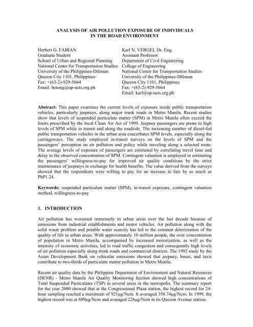
Abstract: This paper examines the current levels of exposure inside public transportation
vehicles, particularly jeepneys, along major trunk roads in Metro Manila. Recent studies
show that levels of suspended particulate matter (SPM) in Metro Manila often exceed the
limits prescribed by the local Clean Air Act of 1999. Jeepney passengers are prone to high
levels of SPM while in transit and along the roadside. The increasing number of diesel-fed
public transportation vehicles in the urban area exacerbates SPM levels, especially along the
carriageways. The study employed in-transit surveys on the levels of SPM and the
passengers’ perception on air pollution and policy while traveling along a selected route.
The average levels of exposure of passengers are estimated by correlating travel time and
delay to the observed concentration of SPM. Contingent valuation is employed in estimating
the passengers’ willingness-to-pay for improved air quality conditions by the strict
maintenance of jeepneys in exchange for health benefits. The value derived from the surveys
showed that the respondents were willing to pay for an increase in fare by as much as
PhP1.24.
Keywords: suspended particulate matter (SPM), in-transit exposure, contingent valuation
method, willingness-to-pay
1. INTRODUCTION
Air pollution has worsened immensely in urban areas over the last decade because of
emissions from industrial establishments and motor vehicles. Air pollution along with the
solid waste problem and potable water scarcity has led to the constant deterioration of the
quality of life in urban areas. With approximately 10 million people, the over concentration
of population in Metro Manila, accompanied by increased motorization, as well as the
intensity of economic activities, led to road traffic congestion and consequently high levels
of air pollution especially along trunk roads and commercial districts. The 1992 study by the
Asian Development Bank on vehicular emissions showed that jeepney, buses, and taxis
contribute to two-thirds of particulate matter pollution in Metro Manila.
Recent air quality data by the Philippine Department of Environment and Natural Resources
(DENR) - Metro Manila Air Quality Monitoring Section showed high concentrations of
Total Suspended Particulates (TSP) in several areas in the metropolis. The summary report
for the year 2000 showed that at the Congressional Plaza station, the highest record for 24hour
sampling reached a maximum of 921µg/Ncm. It averaged 358.74µg/Ncm. In 1999, the
highest record was at 699µg/Ncm and averaged 226µg/Ncm in its Quezon Avenue station.

Human exposure to motor vehicle emissions is greater in urban areas as compared to rural
areas, primarily because cities have more roadways, parking garages, and street canyons
where people may be exposed to high pollutant concentrations due to motor vehicle
emissions (Schwela and Zali, 1999). Variations in pollutant concentration are observed in
different microenvironments (inside buildings, inside homes, inside vehicles, along
roadways, etc.) in the urban area. Individuals in the roadside environment and in-transit are
both exposed to pollutants; they vary with the amount of concentration and the length of
exposure. Several studies have already confirmed the health effects of air pollutants on the
exposed public. Observed effects may be an aggravation of existing respiratory diseases,
disruption of physiological processes or physical inconveniences to the affected population.
The number of people exposed to air pollutants from motor vehicles depends upon the extent
to which a country is motorized (Schwela and Zali 1999). The number of registered motor
vehicles in Metro Manila as shown by the Land Transportation Office statistics is at an
increasing trend with a very high rate, the number of registered vehicles by fuel type shows
that diesel-run vehicles have increased by 613% and gas-run vehicles by 115% from 1980 to
1999.
There have been few studies investigating in-transit levels of SPM and other pollutants. The
California Air Resources Board has posted a summary of the study “Measuring
Concentrations of Selected Air Pollutants inside California Vehicles”. This study was
conducted to characterize the concentration levels of selected pollutants inside commuting in
the Sacramento and Los Angeles areas in California. The results showed relatively higher
levels of all pollutants measured as compared to ambient concentrations as taken from the
mean of commutes in Sacramento and Los Angeles.
The health of passengers and pedestrians can be adversely affected as a result of their
constant exposure to high levels of air pollutants. Majority of the population in Metro
Manila rely heavily on public transportation and spends a considerable amount of time
traveling along congested roadways. The purpose of this study is to evaluate the levels of
exposure to SPM of commuters in major trunk roads in Metro Manila. The study also aims
to investigate the factors influencing in-transit levels of SPM. Specifically, the research aims
to:
• measure the amount of typical SPM concentration inside public vehicles during peak
hours along key trunk roads in Metro Manila
• estimate the length of time a commuter is exposed to varying concentration of SPM
• compare in-transit concentration to ambient concentration of SPM
• investigate the feasibility of a policy aiming to reduce vehicle-generated emissions
Figure 1 shows the relationship of factors affecting air pollution in the transportation
environment. This study is focused on air pollution, particularly SPM, from motor vehicles.
The jeepney is selected as the representative public transportation mode, since according to
the Metro Manila Urban Transportation Integration Study (MMUTIS, 1996), 62% of the
respondents use the jeepney to reach their destination, making the jeepney a major mode of
public transportation in the urban area. The jeepney is a paratransit vehicle sitting 18-20
passengers, with a second-hand truck diesel engine.
Air pollutants from motor vehicles are greatly dependent on meteorological conditions such
as wind velocity, temperature, and humidity and also the way these pollutants interact with
the elements. This study focuses on in-transit levels of SPM concentration. The behavior of

these pollutants inside vehicles is dependent on the vehicles’ ventilation characteristics as
affected by the ambient concentration but does not follow the dispersion of ambient air
pollutants. The health effects of air pollution on passengers may be deduced from the
investigation of their travel behavior, socio-economic status and the observed levels of
exposure.
Industries Motor Vehicles
Other sources
Figure 1. Conceptual Framework of the Study
The succeeding parts of this paper include the analysis of jeepney passengers’ daily
exposure to suspended particulate matter, followed by the multivariate analysis of the
passengers’ willingness-to-pay for air quality improvement. Furthermore, the proposed
strategy to improve air quality in the road environment would be discussed as per the results
of the willingness-to-pay analysis.
2. ANALYSIS OF INDIVIDUAL EXPOSURE TO SPM
2.1 Route Selection
Air
Pollution
Dispersion
In-transit Roadside
Concentration
Exposure length
Health Effects
Traffic Flow
Meteorological Forces
Travel Behavior
Community Perception
Based from MMUTIS (MMUTIS, 1996) data, one of the route that have a high volume of
passengers per day was identified as coming from the northern part of Quezon City, along
Commonwealth Avenue, Quezon Avenue, España Avenue towards the southwest to Taft
Avenue in the heart of Manila. The jeepney route selected started from Philcoa bus and
jeepney stop, passing the stretch of Quezon Avenue and España Avenue, over Quezon

Bridge and finally to Taft Avenue ending in T.M. Kalaw Avenue. The route from Philcoa to
T.M. Kalaw Avenue was measured to be 11.61 km, while the return trip measured 11.85 km.
Figure 2. Study Area and Survey Route
The high volume of jeepneys along this route was also indicative of the high levels of SPM
emitted by diesel engines. The “Air Pollution Survey Using Filter Badge in Metro Manila”
(1998) obtained data on traffic volume along Quezon Avenue and España Avenue. The
jeepney traffic volume along Quezon Avenue had an average of 153 jeepneys/hr, while
España Avenue had 400 jeepneys/hr for both directions.
Ambient monitoring stations for SPM may not be found in all parts of the route, however,
the DENR-NCR Air Quality Monitoring Section has one station along Quezon Avenue as
released from their summary report for 1999. The summary shows that it had an annual
average of 226µg/Ncm for 24-hour sampling of Total Suspended Particles, nearing the limit
of 230µg/Ncm for 24-hour sampling.
2.2 SPM Count, Travel Time and Delay Survey
A surveyor was tasked to record the readings of SPM count cumulatively per minute starting
from the time the jeepney was boarded on Philcoa bus/jeepney stop. The Sibata® Digital
Dust Indicator LD-3 was used as the measuring device. Simultaneously, another surveyor
records travel time and delay starting when the jeepney was boarded. Both measurements
stop when T.M. Kalaw Avenue was reached, this was considered as one run with starting
time of approximately 7:00 am. The second run started from T.M. Kalaw Avenue and ended
in Philcoa, which is the return trip of the jeepney. Another set of runs started in the
afternoon, approximately starting at 4:00 pm from Philcoa. The dates for the survey runs
were all weekdays, February 8, 9 and 12, 2001 respectively, so as to capture the bulk of
passenger trips. The actual time of observations during the morning and afternoon runs are
presented in Table 1.

Table 1. Start and End Time of the Runs to and from Philcoa to Kalaw
ug/ Ncm
Philcoa - Kalaw Kalaw - Philcoa
AM PM AM PM
2/8/2001 7:12 - 8:17 4:13 - 5:12 8:29 - 9:14 5:33 - 6:50
2/9/2001 6:51 - 7:53 4:18 - 5:21 7:59 - 8:55 5:27 - 6:34
2/12/2001 7:05 - 8:09 4:03 - 5:20 8:17 - 9:07 5:21 - 6:42
2.3 SPM Exposure and Travel Time Analysis
The level of exposure of individuals in the road environment is greatly dependent on the
amount of time they spend on the road environment, along the roadside and in-transit. The
total daily exposure of an individual to air pollution is the sum of the separate contacts to air
pollution experienced by the individual as he pass through a series of environments (also
called microenvironments) during the course of the day (e.g. at home, while commuting, in
the streets, etc.). Exposure in each of these environments can be estimated as the product of
the pollutant concentration and the time spent in specific microenvironments (WHO, 2000).
This paper uses this concept in estimating the total exposure of the affected population using
public transportation. The general form of the equation used to calculate time-weighted
integrated exposure is:
J
Εί = Σ Cj tij (1)
j
where Εί is the time-weighted integrated exposure for person i over the specified time
period; Cj is the pollutant concentration in micro-environment j; and J is the total number of
microenvironments that person i moves through the specified time period (Sexton and Ryan,
1988). A microenvironment is defined as a three-dimensional space where the pollutant
level at some specified time is uniform or has constant statistical properties. Outdoors in a
specific community, inside a motor vehicle, and inside a particular residence are examples
of locations that can be defined, under appropriate conditions, microenvironments (Sexton
and Ryan, 1988).
The results of the observed values of SPM concentrations are presented in the following
figures. The graphical representations of the runs show similarities with the trends of SPM
concentrations by time. Figures 3 and 4 show the observed SPM concentrations inside the
jeepney from Philcoa to T.M. Kalaw. Figures 5 and 6 show the observed SPM
concentrations inside the jeepney from T.M. Kalaw to Philcoa. The concentrations are
presented with respect to the travel time per minute.
2500
2000
1500
1000
500
0
0
4
8
12
16
20
24
28
32
36
40
44
travel time in m inutes
48
52
56
60
64
8-Feb
9-Feb
12-Feb
Figure 3. Observed SPM Concentration from Philcoa to T.M. Kalaw Avenue
during the Morning Peak Runs

ug/ Ncm
ug/ Ncm
900
800
700
600
500
400
300
200
100
0
0
1800
1600
1400
1200
1000
800
600
400
200
0
0
4
3
6
travel time in minutes
travel time in minutes
8
12
16
20
24
28
32
36
40
44
48
52
56
60
64
68
72
76
9
12
15
18
21
24
27
30
33
36
39
42
45
48
51
54
8-Feb
9-Feb
12-Feb
Figure 4. Observed SPM Concentration from Philcoa to T.M. Kalaw Avenue
during the Afternoon Peak Runs
ug/ Ncm
1200
1000
800
600
400
200
0
0
5
10
15
20
25
30
35
40
45
50
55
60
travel time in minutes
65
70
75
80
8-Feb
9-Feb
12-Feb
Figure 5. Observed SPM Concentration from T.M. Kalaw Avenue to Philcoa
during the Morning Peak Runs
8-Feb
9-Feb
12-Feb
Figure 6. Observed SPM Concentration from T.M. Kalaw Avenue to Philcoa
during the Afternoon Peak Runs
The average travel time was computed from the morning and afternoon runs to and from
Philcoa to T.M. Kalaw Avenue. The variations of travel speed from Philcoa to T.M. Kalaw
Avenue in the morning and in the afternoon can be seen in Figures 7 and 8 showing the
mean travel speed and mean running speed of the runs in the morning and in the afternoon
with respect to the distance covered.
The average travel time was computed from all the runs separately per direction and time of
day. Summary of the average travel time is presented in Table 2. It was observed that runs
during the afternoon took a relatively longer time than the morning runs. All runs were done
during peak hours but it is evident that travel time was longer during the afternoon peak
hours.

Speed (kph)
Speed (kph)
35
30
25
20
15
10
5
0
35
30
25
20
15
10
5
0
AM Philcoa - Kalaw Runs
0 2 4 6 8 10 12 14
Distance Covered (km)
travel speed mean travel speed mean running speed
AM Kalaw to Philcoa Runs
0 2 4 6 8 10 12 14
Distance Covered (km)
travel speed mean travel speed mean running speed
PM Philcoa - Kalaw Runs
Philcoa - Kalaw Kalaw - Philcoa
AM PM AM PM
2/8/2001 65 59 45 77
2/9/2001 62 63 56 67
2/12/2001 64 77 50 81
Average 64 66 50 75
Speed (kph)
35
30
25
20
15
10
5
0
0 2 4 6 8 10 12 14
Distance Covered (km)
travel speed mean travel speed mean running speed
Figure 7. Travel Speed-Distance Diagram for AM and PM Runs from
Philcoa to T.M. Kalaw Avenue
Speed (kph)
30
25
20
15
10
5
0
PM Kalaw - Philcoa Runs
0 2 4 6 8 10 12 14
Distance Covered (km)
travel speed mean travel speed mean running speed
Figure 8. Travel Speed-Distance Diagram for AM and PM Runs from
T.M. Kalaw Avenue to Philcoa
Table 2. Summary of Travel Time to and from Philcoa to T.M. Kalaw Avenue in Minutes
The authors used different sections along the route with the observed delays to compute the
average travel speed and running speed for each section. The sections identified were mostly
between signalized intersections along the route.
Figures 9 to 12 show the variation in the measured SPM concentration with respect to the
different sections along the route. There is high variation in the observed section
concentrations. A probable reason is that the different sections chosen along the route are
not equidistant from each other, however, as shown in the graphs, there are still sections that
have very high disparities among the observed levels for the different runs. This signifies
that the distances between the specified sections do not directly affect SPM concentrations.
The sensitivity of the measuring instrument to SPM from direct emissions of jeepneys along
the route is the reason for these erratic concentrations of SPM inside the jeepney while in
transit. Smoke-belching vehicles near the ridden jeepney or the smoke emitted by the ridden
jeepney itself increases the readings taken from the measuring instrument. Nonetheless, the

observed concentrations of SPM are very high compared to ambient concentrations.
Ambient concentrations are measured on a short-term and long-term basis with short-term
monitoring equal to a 24-hour sampling period and long-term monitoring equal to an annual
sampling period. The observed concentrations of SPM inside the jeepney and while in
transit, only stands for the amount of time an individual is in transit.
ug/Ncm
ug/Ncm
2000
1800
1600
1400
1200
1000
800
600
400
200
0
700
600
500
400
300
200
100
0
1 3 5 7 9 11 13 15 17 19 21 23 25 27 29
sections
1 3 5 7 9 11 13 15 17 19 21 23 25 27 29
sections
8-Feb
9-Feb
12-Feb
Figure 9. Average SPM Concentration by Section from Philcoa to T.M. Kalaw Avenue
during the Morning Peak Runs
ug/Ncm
1400
1200
1000
800
600
400
200
0
1 3 5 7 9 11 13 15 17 19 21 23 25 27 29
sections
8-Feb
9-Feb
12-Feb
Figure 10. Average SPM Concentration by Section from Philcoa to T.M. Kalaw Avenue
during the Afternoon Peak Runs
8-Feb
9-Feb
12-Feb
Figure 11. Average SPM Concentration by Section from T.M. Kalaw Avenue to Philcoa
during the Morning Peak Runs

ug/Ncm
1000
900
800
700
600
500
400
300
200
100
0
1 3 5 7 9 11 13 15 17 19 21 23 25 27 29
sections
Philcoa - Kalaw Kalaw - Philcoa
AM PM AM PM
8-Feb 55.94 7.72 19.47 13.01
9-Feb 18.08 12.14 14.24 14.16
12-Feb 26.53 10.59 18.07 18.81
Average 33.52 10.15 17.26 15.33
8-Feb
9-Feb
12-Feb
Figure 12. Average SPM Concentration by Section from T.M. Kalaw Avenue to Philcoa
during the Afternoon Peak Runs
The travel time data and the observed values of SPM concentrations while in transit were
used in estimating the levels of exposure of individuals while in transit. The 24-hour timefraction
of the time spent in each section throughout the route was used to get the levels of
exposure of individuals while inside the jeepney and in transit.
Using equation (1), the levels of exposure of individuals inside jeepneys were computed.
The average values are shown in Table 4.
Table 3. Estimated Levels of Exposure of Passengers inside Jeepneys (µg/Ncm)
Studies regarding time-activity patterns of individuals help in the over-all estimation of an
integrated exposure assessment to air pollution for a 24-hour period. In a study by Szalai
(1992) and Chapin (1974), they presented a 24-hour activity pattern for an individual. Both
studies found that on most days people are inside their residences for an average of 65 to 70
percent of the time, and indoors at home, work, or elsewhere for more than 90 percent of the
time. Although these values vary with age, gender, occupation, socio-economic status, and
day of the week, it has become clear that indoor microenvironments must be taken into
account for a realistic assessment of exposure to many air pollutants (Sexton and Ryan,
1988). Correspondingly, the concentration of respirable suspended particles was used to
compute exposure levels. The study emphasized the importance of evaluating in-transit
exposure since the results show that in-transit exposure contributes to 15% of the exposure
for a 24-hour integrated period. Also, in-transit levels of respirable suspended particle
concentrations were observed to be higher than other microenvironments. Respirable
suspended particles, also synonymous with suspended particulate matter are those particles
that can be inhaled by humans.
The level of exposure of the individual on each section of the trip was computed from the
observed concentration of SPM and the time spent as shown in Figure 13. This was done in
order to investigate the amount of exposure an individual takes along the trip.

ug/Ncm
4.5
4
3.5
3
2.5
2
1.5
1
0.5
0
0 5 10 15 20 25 30 35
sections
Parameter Intercept SECTTIME
Estimates 0.18613491 0.003528114
St. Error 0.04709825 0.000287613
t-statistic 3.95205562 12.2668888
p-level 9.3653E-05 4.81378E-29
8-Feb
9-Feb
12-Feb
Figure 13. Levels of Exposure by Section along the Philcoa to Kalaw Route (AM Runs)
The results of the surveys show that the average travel time to and from Philcoa to T.M.
Kalaw Avenue is approximately 1 hour. For the number of people who frequently use the
Philcoa to T.M. Kalaw Avenue route, the time fraction they spend in transit is equal to 0.08
or 2 hours. The observed SPM concentrations and the time spent showed that average levels
of exposure for one trip reached a maximum of 33.52µg/Ncm and a low of 10.15µg/Ncm
(Table 3). This value is only representative of the individual’s exposure to SPM while intransit.
The daily limit set by the local Clean Air Act of 1999 is pegged at 230µg/Ncm for shortterm
monitoring of suspended particulate matter. Considering the results of the observed
values of SPM concentrations while in transit, the possible levels of exposure yield a high
amount. The average travel time for the Philcoa to T.M. Kalaw Avenue route was observed
to be 2 hours for a round trip and the average level of SPM, regardless of time and direction
is 19.07µg/Ncm. The exposure level is equal to 17.48µg/Ncm. This is just equivalent to the 2
hours the individual has spent while traveling.
The relationship of SPM and exposure with regard to the travel time and delay study were
analyzed by regressing the SPM concentration and the computed exposure of the individual
while in transit on variables such as running speed, running time, travel speed, and travel
time. The regression result showed a better model by using the exposure data as the
dependent variable as compared to using the observed SPM concentrations.
The variable with the most relevant relationship was found to be the travel time for each
section indicated by SECTTIME. Other variables such as running speed, distance, travel
speed, and delay showed very little significance in the regression. Results of the regression
are shown below:
Table 4. Regression Results for Exposure and Travel Time
Despite the low R 2 of 0.30, this model yielded the highest measure of significance as
compared with and in combination to the other variables such as, running speed, running
time, delay and travel speed. The positive sign of the SECTTIME variable indicates that as
the travel time for a section increases, the exposure of the individual also increases. The

elevance of this regression analysis is that the authors were able to look into the possible
factors influencing SPM concentration while in transit. The regression result was able to
conclude that the concentration of SPM is not affected by the running speed and delay of the
jeepney.
3. WILLINGNESS-TO-PAY FOR THE IMPROVEMENT OF AIR QUALITY
Establishing the fact that passengers are exposed to higher levels of SPM as previously
conceived by ambient monitoring, the authors employed a face-to-face interview on the
jeepney passengers in transit and while waiting for a ride in order to know their perception
and willingness-to-pay for improved air quality.
3.1 Data Collection
Simultaneous with the SPM and travel time and delay survey, another surveyor was tasked
to conduct a face-to-face interview survey of passengers inside the jeepney while traveling
the route. The passenger’s travel behavior, socio-economic status, perception on health
effects of SPM, perception on air quality inside jeepneys and on the roadside environment,
and willingness-to-pay was gathered. Another face-to-face interview survey on jeepney
passengers was done on June 13, 2001 at the Philcoa bus/jeepney stop. This time the target
respondents were the people waiting for a jeepney ride.
3.2 Contingent Valuation Questionnaire
The discrete-response contingent valuation question introduces the relationship of motor
vehicle emissions to human health, particularly suspended particulate matter. The
interviewer clearly explained to the respondent that SPM emissions by jeepneys and other
diesel-fed engines could affect their health. A strategy by the government by mandating
jeepney drivers/operators to regularly comply with a monthly check-up of their vehicles with
the proper authorities was also introduced to the respondent. Then the interviewer explains
that the drivers/operators may not be able to comply with this policy due to their financial
inadequacy.
The interviewer then asked the question on their willingness-to-pay for an additional
increase in fare. For the first survey, the initial bid was fixed at PhP1.00. If the reply was
‘yes’ then interviewer follows it up with PhP2.00 bid and if the reply was ‘no’, the
interviewer offers a lower cost, PhP0.50. The second survey employed the draw card
technique in order to eliminate the initial bid bias. The first bid was randomly chosen by the
respondent from a set of cards, after which, their reply was elicited. A higher bid was again
offered by the interviewer, if the reply is ‘yes’ and a lower bid, if otherwise. The second bid
was still drawn from the prepared set of cards.
3.3 Multivariate Analysis
Information regarding the individual’s travel behavior, socio-economic status, air quality
perception, perceived effect on human health, and willingness-to-pay in order to help
regulate SPM emissions by jeepneys, were analyzed through a logit regression model. Table
5 shows the profile of the respondents from the interview-survey. Consequently, these also
serve as the variables used in the regression model so as to investigate the possible effect of
these variables in the individuals’ decision to pay for improved air quality.

Table 5. Profile of Respondents
Variables Description Mean St. Dev.
CHOICE Dependent Variable; 1=Yes, 0=No 0.375 0.485
INITBID Initial bid; P0.5, P1, P1.50, P2, P2.50, P3, P3.50 1.610 0.663
GEN Gender; 1=Male, 0=Female 0.510 0.501
STAT Status; 1=Single, 0=Married 0.550 0.499
AGE Age; continuous data 28.425 10.696
CAROWN Car ownership; 1=with car, 0=without car 0.158 0.366
EDUC Educ. Attainment; 1=Elem., 2=Sec.,3=Vocational, 4=College, 5=Post College 2.900 0.962
HINC Household Income; 1=

xz = represents the different combinations yy, yn, ny, and nn,
SP = stated preference/ answer of the respondents
The median willingness-to-pay may be computed from changing V(1, Y-C)-V(0,Y) in the
logit formula (2) to ∆V(C), in order to reflect the variations in cost. Equation 2 may be
transformed to the formula below in deriving the median willingness-to-pay.
C* = exp (α / β) (4)
where C* = median cost of the responses
α and β = parameter estimates
The median was used as the measure of central tendency representing the data because the
bids were already preset, meaning it is not affected by extreme values in the response
distribution. The mean is the conventional measure in benefit-cost analysis and from a
statistical point of view, more sensitive than the median, however, the median may be more
realistic in a world where decisions are based on voting and there is a concern for the
distribution of benefits and costs (Hanneman, 1999). The results of the maximum likelihood
estimation are shown below.
Table 6. Summary of Regression
Survey 1 Survey 2 HHoldInc1 HHoldInc2 HHoldInc3
Parameter α β α β α β α β α β
Estimates 0.36 1.66 0.19 1.45 -0.47 1.26 -0.02 1.89 0.26 1.21
Standard Error 0.24 0.26 0.16 0.16 0.33 0.32 0.22 0.27 0.21 0.18
t-statistic 1.45 6.45 1.21 9.28 -1.43 3.91 -0.10 7.05 1.25 6.64
No. of Samples
Log of Likelihood =
C* =
Note:
61 139 40 77
80
-327.335 -860.839 -194.763 -433.145 -456.245
1.24 1.14 0.69 0.99 1.24
HHoldInc1 = household income below 10,000 pesos/month
HHoldInc2 = household income 10,001-20,000 pesos/month
HHoldInc3 = household income greater than 20,000 pesos/month
Survey 1 was done simultaneously with the SPM and travel time survey. The respondents
were inside the jeepney while in-transit. Survey 2, on the other hand, was conducted on
passengers waiting for a jeepney along Philcoa. HHoldInc1, HHoldInc2 and HHoldInc3
stands for the aggregated respondents from survey 1 and 2, segmented according to the
household income of the respondents.
The log of likelihood of the model is indicative of its significance and a higher probability of
the dependent variable to occur in the sample. The log of likelihood is also dependent on the
robustness of the data; the higher the value means the larger the sample size. The low tstatistics
of α indicates that it is not that relevant at the 95% significance level.
Using the parameter estimates derived from the maximum likelihood estimation, the
probability that the respondents will pay for the increase in fare was computed. Figure 13
shows a comparison of the two surveys, with the first survey having a slightly higher
probability curve than the second survey. Although the disparity between the two is not big,
it can be inferred that the respondents of the first survey, done inside the jeepney and in
transit, obtained a higher median value for their willingness-to-pay and probability curve.
Their direct exposure to higher SPM levels during the interview could affect the results.

Probability that Respondents will pay
at the indicated fee
Probability that respondents will pay
at the indicated fee
1
0.9
0.8
0.7
0.6
0.5
0.4
0.3
0.2
0.1
0
1
0.9
0.8
0.7
0.6
0.5
0.4
0.3
0.2
0.1
0
0 0.5 1 1.5 2 2.5 3 3.5 4
Fare Increase (pesos/trip )
Survey 1 Survey 2
Figure 13. Probability of Respondents Paying for Improved Air Quality at the Indicated Fee
To be able to investigate the willingness-to-pay with respect to the economic status of the
respondents with their willingness-to-pay, the probability curves for different income groups
were also graphed as shown in Figure 14.
0 0.5 1 1.5 2 2.5 3 3.5 4
Fare Increase (pesos/trip)
HH income below 10,000 pesos/month
HH income 10,001-20,000 pesos/month
HH income greater than 20,000 pesos/month
Figure 14. Probability of Households Paying for Improved Air Quality at the Indicated Fee
The income groups were aggregated into three categories, as shown in the graph. As
expected, the lowest income group obtained the lowest probability curve and median
willingness-to-pay. Also, the highest income group had the highest median value and posted
a high probability even at higher bids of fare increase. Surprisingly though, the household
income group of 10,001-20,000 pesos/month surpassed the household income group of
greater than 20,000 pesos/month when it came to the lowest bid, which is PhP0.25.
4. CONCLUSIONS AND RECOMMENDATIONS
The study’s analysis on in-transit levels of suspended particulate matter showed higher
levels of SPM while in transit along a major trunk road, compared to the regular ambient
concentrations in Metro Manila. Also, the levels of exposure of an individual were presented
while in transit. The time-weighted 24-hour integrated exposure showed that the exposure
levels are high considering the time fraction that an individual spends in transit for a day.

Given the current levels of SPM concentrations as reported by ambient monitoring stations
of the Department of Environment and Natural Resources, roadside and area concentrations
of SPM may also be very high, hence, further increasing the exposure of individuals to SPM
for a 24-hour period, exceeding the limits prescribed.
The results of the contingent valuation on the respondents’ willingness to pay have shown
that the respondents were willing to pay for as much as a PhP1.24 pesos increase in fare for
the improvement of air quality. A possible application of the policy would mean that the
current minimum fare, which is PhP4.00, could be increased to a high of PhP5.24 as per the
result of the survey. The results showed that the passengers in-transit have given a relatively
higher cost than the respondents along the roadside waiting for a ride. This was probably due
to the fact they were exposed to higher SPM levels during the interview-survey itself. The
probability curve for the household income showed that the lower income group was more
hesitant to pay for improved air quality than the higher income groups, following the
economic theory.
Strategy is important for the success of any policies that the government may implement.
Without proper education of the public regarding the health hazards posed by air pollution,
the policy may not be as effective as expected. The values generated are considered as the
value an individual is willing to pay per trip, in exchange for cleaner air, hence, better
health. Aggregating this value for a one-day trip to and from work in a public transportation
mode, it can be derived that an individual regularly riding a jeepney everyday may actually
shell out an increase of approximately PhP2.50 per day or PhP50.00 per month for improved
air quality. Moreover, implementation techniques should also be explored. A gradual
increase in fare may be more favorable than an abrupt one.
Further studies should aim to investigate traffic volume and temperature as a factor in the
observed levels of exposure to SPM in-transit. Also, health effects of SPM towards public
transport passengers and other carriageway users should be further investigated in Metro
Manila in order to correlate the observed levels of exposure with the incidences of
respiratory diseases, aggravations of diseases, and mortality and morbidity rates in the
metropolis. Further studies regarding levels of concentration of SPM and other pollutants in
different microenvironments would be vital in the assessment of the total exposure of an
individual per day. Possible health effects may then be more accurately anticipated and
remedied. In terms of the publics willingness-to-pay, other fee collection techniques may
also be looked at, aside from increasing the transportation fare.
ACKNOWLEDGMENT
The authors would like to extend their gratitude to the Institute of Behavioral Sciences of
Japan and the National Center for Transportation Studies of the University of the Philippines
– Diliman, to Dr. Shoshi Mizokami, JICA Visiting Professor to NCTS 2000-2001 and
Professor of Kumamoto University, Japan for teaching the contingent valuation method to
NCTS graduate students and faculty. Also, sincere gratitude is given to Prof. Tetsuo Yai,
Mr. Mitsuhata, and Mr. Hirata of the Tokyo Institute of Technology Planning Laboratory for
the continuing study on the transportation environment in Metro Manila. This joint research
between Tokyo Institute of Technology, Shibaura Institute of Technology and the University
of the Philippines National Center for Transportation Studies (UP-NCTS) is a part of the
research project entitled “Impact Analysis of Policies for Development and Environmental

Conservation in the Philippines”, named as the JSPS Manila Project, commencing from
1997 until 2002, and funded by The Japan Society for the Promotion of Science.
REFERENCES
Japan Society for the Promotion of Science (1998) ‘Air Pollution Survey Using Filter
Badge in Metro Manila’
Asian Development Bank (1992) Vehicular Emission Control Planning in Metro Manila,
Final Report, July 1992
Hanemann, Michael and Barbara Kanninen. (1999) “Statistical Analysis of Discrete-
Response CV Data”, Valuing Environmental Preferences: Theory and Practice of the
Contingent Valuation Method in the US, EU and Developing Countries, Oxford
University Press, New York.
Philippine Department of Environment and Natural Resources (DENR) – National Capital
Region (NCR) Air Quality Monitoring Section - Summary Reports for TSP 1999 and 2000
Larssen, S. et al. (1997) Urban Air Quality Management Strategy in Asia: Metro
Manila Report. Technical Paper No. 380, The World Bank, Washington, D.C.
Metro Manila Urban Transportation Integration Study (MMUTIS) Draft Final Report.
(1998).
Mitsuhata, Futoshi. (2001) Developing a System for Transportation Policy Assessment for
SPM Reduction Incorporating the Public Perception on the Environment (Master’s Thesis).
Department of Built Environment, Tokyo Institute of Technology, Japan.
Schwela, Dietrich and Olivier Zali ed. (1999) Urban Traffic Pollution. E & FN Spon,
Great Britain.
Sexton, Ken and P. Barry Ryan. (1988) Assessment of Human Exposure to Air Pollution:
Methods, Measurements, and Models. In A.Y. Watson, R.R. Bates, D. Kennedy (eds.) Air
Pollution, the Automobile and Public Health. Health Effects Institute, National Academy
Press, Washington D.C.
Teodoro, R.V. and Villoria, Jr., O. (1997) Empirical analysis on the relationship between air
pollution and traffic flow parameters. Proceedings of the Eastern Asia Society for
Transportation Studies 2nd Conference, Volume 1, Seoul, Korea, 29-31, October 1997.
Vergel, Karl, et.al. (2001) Micro-Scale Analysis of the Transportation Environment in
Metro Manila. (for publication and presentation) 9th World Conference on Transportation
Research, July 22-28, 2001.
World Health Organization (WHO). (2000) Guidelines for Air Quality. Geneva,
Switzerland.