Introduction to Local Level Model and Kalman Filter
Introduction to Local Level Model and Kalman Filter
Introduction to Local Level Model and Kalman Filter

You also want an ePaper? Increase the reach of your titles
YUMPU automatically turns print PDFs into web optimized ePapers that Google loves.
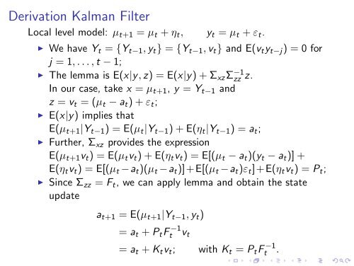
Derivation <strong>Kalman</strong> <strong>Filter</strong><br />
<strong>Local</strong> level model: µt+1 = µt + ηt, yt = µt + εt.<br />
◮ We have Yt = {Yt−1, yt} = {Yt−1, vt} <strong>and</strong> E(vtyt−j) = 0 for<br />
j = 1, . . . , t − 1;<br />
◮ The lemma is E(x|y, z) = E(x|y) + ΣxzΣ −1<br />
zz z.<br />
In our case, take x = µt+1, y = Yt−1 <strong>and</strong><br />
z = vt = (µt − at) + εt;<br />
◮ E(x|y) implies that<br />
E(µt+1|Yt−1) = E(µt|Yt−1) + E(ηt|Yt−1) = at;<br />
◮ Further, Σxz provides the expression<br />
E(µt+1vt) = E(µtvt) + E(ηtvt) = E[(µt − at)(yt − at)] +<br />
E(ηtvt) = E[(µt −at)(µt −at)]+E[(µt −at)εt]+E(ηtvt) = Pt;<br />
◮ Since Σzz = Ft, we can apply lemma <strong>and</strong> obtain the state<br />
update<br />
at+1 = E(µt+1|Yt−1, yt)<br />
= at + PtF −1<br />
t vt<br />
= at + Ktvt; with Kt = PtF −1<br />
t .