Introduction to Local Level Model and Kalman Filter

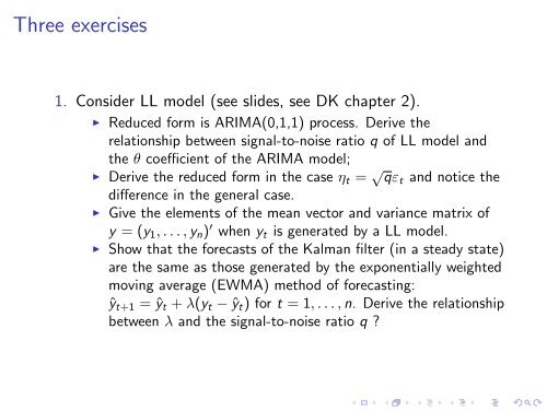
Three exercises
1. Consider LL model (see slides, see DK chapter 2).
◮ Reduced form is ARIMA(0,1,1) process. Derive the
relationship between signal-to-noise ratio q of LL model and
the θ coefficient of the ARIMA model;
◮ Derive the reduced form in the case ηt = √ qεt and notice the
difference in the general case.
◮ Give the elements of the mean vector and variance matrix of
y = (y1, . . . , yn) ′ when yt is generated by a LL model.
◮ Show that the forecasts of the Kalman filter (in a steady state)
are the same as those generated by the exponentially weighted
moving average (EWMA) method of forecasting:
ˆyt+1 = ˆyt + λ(yt − ˆyt) for t = 1, . . . , n. Derive the relationship
between λ and the signal-to-noise ratio q ?