Pythagorean-hodograph curves in Euclidean spaces of dimension ...
Pythagorean-hodograph curves in Euclidean spaces of dimension ...
Pythagorean-hodograph curves in Euclidean spaces of dimension ...

You also want an ePaper? Increase the reach of your titles
YUMPU automatically turns print PDFs into web optimized ePapers that Google loves.
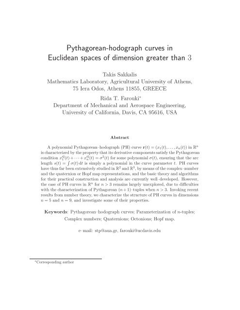
<strong>Pythagorean</strong>-<strong>hodograph</strong> <strong>curves</strong> <strong>in</strong><br />
<strong>Euclidean</strong> <strong>spaces</strong> <strong>of</strong> <strong>dimension</strong> greater than 3<br />
Takis Sakkalis<br />
Mathematics Laboratory, Agricultural University <strong>of</strong> Athens,<br />
75 Iera Odos, Athens 11855, GREECE<br />
Rida T. Farouki ∗<br />
Department <strong>of</strong> Mechanical and Aerospace Eng<strong>in</strong>eer<strong>in</strong>g,<br />
University <strong>of</strong> California, Davis, CA 95616, USA<br />
Abstract<br />
A polynomial <strong>Pythagorean</strong>–<strong>hodograph</strong> (PH) curve r(t) = (x1(t),... ,xn(t)) <strong>in</strong> Rn is characterized by the property that its derivative components satisfy the <strong>Pythagorean</strong><br />
condition x ′2<br />
1 (t)+···+x′2 n (t) = σ2 (t) for some polynomial σ(t), ensur<strong>in</strong>g that the arc<br />
length s(t) = σ(t)dt is simply a polynomial <strong>in</strong> the curve parameter t. PH <strong>curves</strong><br />
have thus far been extensively studied <strong>in</strong> R2 and R3 , by means <strong>of</strong> the complex–number<br />
and the quaternion or Hopf map representations, and the basic theory and algorithms<br />
for their practical construction and analysis are currently well–developed. However,<br />
the case <strong>of</strong> PH <strong>curves</strong> <strong>in</strong> Rn for n > 3 rema<strong>in</strong>s largely unexplored, due to difficulties<br />
with the characterization <strong>of</strong> <strong>Pythagorean</strong> (n+1)–tuples when n > 3. Invok<strong>in</strong>g recent<br />
results from number theory, we characterize the structure <strong>of</strong> PH <strong>curves</strong> <strong>in</strong> <strong>dimension</strong>s<br />
n = 5 and n = 9, and <strong>in</strong>vestigate some <strong>of</strong> their properties.<br />
Keywords: <strong>Pythagorean</strong>–<strong>hodograph</strong> <strong>curves</strong>; Parameterization <strong>of</strong> n-tuples;<br />
∗ Correspond<strong>in</strong>g author<br />
Complex numbers; Quaternions; Octonions; Hopf map.<br />
e–mail: stp@aua.gr, farouki@ucdavis.edu
1 Introduction<br />
A polynomial curve r(t) = (x1(t), . . .,xn(t)) <strong>in</strong> R n is a <strong>Pythagorean</strong>–<strong>hodograph</strong> (PH) curve<br />
if its <strong>hodograph</strong> (derivative) r ′ (t) = (x ′ 1(t), . . .,x ′ n(t)) has components that satisfy, for some<br />
polynomial σ(t), the <strong>Pythagorean</strong> condition<br />
x ′2<br />
1 (t) + · · · + x′2 n (t) = σ2 (t) . (1)<br />
Consequently, the parametric speed |r ′ (t)| = ds/dt — i.e., the rate <strong>of</strong> change <strong>of</strong> arc length<br />
s with respect to the parameter t — is just a polynomial (rather than the square root <strong>of</strong> a<br />
polynomial) <strong>in</strong> t. This feature endows PH <strong>curves</strong> with many advantageous algorithms for<br />
geometric design, motion control, animation, path plann<strong>in</strong>g, and related applications.<br />
PH <strong>curves</strong> were first <strong>in</strong>troduced [10] <strong>in</strong> R 2 us<strong>in</strong>g a simple characterization for <strong>Pythagorean</strong><br />
polynomial triples, that can be conveniently expressed <strong>in</strong> terms <strong>of</strong> a complex–variable model<br />
[3, 8, 9]. Subsequently, PH <strong>curves</strong> <strong>in</strong> R 3 were characterized <strong>in</strong> terms <strong>of</strong> the quaternion and<br />
Hopf map models [2, 6] — which facilitate the identification <strong>of</strong> some <strong>in</strong>terest<strong>in</strong>g special<br />
sub–classes [5, 7, 13]. A further extension <strong>of</strong> the theory <strong>in</strong>volves study <strong>of</strong> the PH condition<br />
(1) under the M<strong>in</strong>kowski (rather than <strong>Euclidean</strong>) metric [14] — i.e., with the + sign before<br />
x ′2 n (t) <strong>in</strong> (1) replaced by a − sign. The study <strong>of</strong> solutions to x′2 1 (t)+x′2 2 (t)−x′2 3 (t) = σ2 (t) <strong>in</strong><br />
the M<strong>in</strong>kowski space R (2,1) is motivated by the desire to exactly reconstruct the boundary<br />
<strong>of</strong> a planar doma<strong>in</strong> from its medial axis transform. Further details on all these different<br />
<strong>Euclidean</strong> and M<strong>in</strong>kowski PH curve <strong>in</strong>carnations may be found <strong>in</strong> [4].<br />
This paper shows that the Hopf model, used to characterize PH <strong>curves</strong> <strong>in</strong> R 2 and R 3 , can<br />
also be generalized to obta<strong>in</strong> characterizations for PH <strong>curves</strong> <strong>in</strong> R 5 and R 9 . The outl<strong>in</strong>e for<br />
the rema<strong>in</strong>der <strong>of</strong> the paper is as follows. Section 2 reviews some basic results concern<strong>in</strong>g<br />
<strong>Pythagorean</strong> (n + 1)–tuples <strong>of</strong> real polynomials, and uses them to extend the theory <strong>of</strong><br />
planar and spatial PH <strong>curves</strong> to R 5 and R 9 (and thereby also R 4 and R 8 ). A one–to–one<br />
correspondence between the regular PH <strong>curves</strong> <strong>in</strong> R n and (equivalence classes <strong>of</strong>) regular<br />
“ord<strong>in</strong>ary” polynomial <strong>curves</strong> <strong>in</strong> R 2n−2 is also established. Section 3, whose results are<br />
<strong>in</strong>dependent from the rest <strong>of</strong> the paper, provides a characterization <strong>of</strong> the conditions under<br />
which two complex, quaternion, or octonion polynomials are constant multiples <strong>of</strong> each<br />
other. These results are then used <strong>in</strong> Section 4 to obta<strong>in</strong> simple criteria identify<strong>in</strong>g l<strong>in</strong>ear<br />
and planar <strong>in</strong>stances <strong>of</strong> higher–<strong>dimension</strong>al PH <strong>curves</strong>. F<strong>in</strong>ally, Section 5 summarizes the<br />
key results <strong>of</strong> this study, and identifies some open problems.<br />
1
2 <strong>Pythagorean</strong> (n + 1)-tuples<br />
We first review some recent results from [15] that are essential to the subsequent analysis.<br />
The construction <strong>of</strong> PH <strong>curves</strong> has thus far been based on the solution <strong>of</strong> the <strong>Pythagorean</strong><br />
condition (1) <strong>in</strong> the cases n = 2 and n = 3. To construct PH <strong>curves</strong> <strong>in</strong> R n when n > 3, it<br />
is essential to characterize all solutions <strong>of</strong> (1) for n > 3.<br />
Let R[t] be the r<strong>in</strong>g <strong>of</strong> univariate real polynomials, and let n ≥ 1. Then a <strong>Pythagorean</strong><br />
(n + 1)–tuple over R[t] is a vector (p1(t), . . .,pn(t), pn+1(t)) ∈ R n+1 [t], such that<br />
p 2 1(t) + · · · + p 2 n(t) = p 2 n+1(t) . (2)<br />
Theorem 4.1 on page 1268 <strong>of</strong> [15], which uses ideas from quadratic forms, gives all solutions<br />
<strong>of</strong> (2) for some special values <strong>of</strong> n. Before stat<strong>in</strong>g it, we need to <strong>in</strong>troduce some notation.<br />
Let R, C, H, and O denote the sets <strong>of</strong> real numbers, complex numbers, quaternions, and<br />
octonions, where we make the identifications C = R 2 , H = R 4 , and O = R 8 .<br />
Now if A is a member <strong>of</strong> one <strong>of</strong> these sets, we denote by A its norm, by A ∗ its conjugate<br />
(such that A ∗ A = AA ∗ = A 2 ), and by Re(A) and Im(A) its real and imag<strong>in</strong>ary parts.<br />
Also, the appropriate (real, complex, quaternion, or octonion) product is imputed whenever<br />
two such elements appear <strong>in</strong> juxtaposition. See the Appendix for a brief review <strong>of</strong> these<br />
ideas <strong>in</strong> the case <strong>of</strong> the quaternions H and the octonions O.<br />
Theorem 2.1 Let A(t), B(t) ∈ R n−1 [t] and c(t) ∈ R[t]. Then, modulo permutations, the<br />
solutions <strong>of</strong> (2) over R[t] <strong>in</strong> the cases n = 2, 3, 5, 9 are <strong>of</strong> the form<br />
(p1, p2, . . .,pn, pn+1) = c (A 2 − B 2 , 2A B ∗ , A 2 + B 2 ) . (3)<br />
Now for k = 1, 2, 4, 8 let Rk denote the set R, C, H, O, and let Rk+1 = R × Rk. A closer<br />
look at (3) reveals that the solution set <strong>of</strong> (2) is an <strong>in</strong>stance <strong>of</strong> the real Hopf fibration<br />
H : Rk × Rk → Rk+1 def<strong>in</strong>ed for α, β ∈ Rk by<br />
H(α, β) = (α 2 − β 2 , 2 αβ ∗ ) . (4)<br />
Indeed, if Rk and Rk+1 are replaced by the correspond<strong>in</strong>g polynomial r<strong>in</strong>gs Rk[t] and Rk+1[t]<br />
we note that c (A 2 − B 2 , 2A B ∗ , A 2 + B 2 ) = c (H(A, B), H(A, B)).<br />
2
2.1 <strong>Pythagorean</strong>–<strong>hodograph</strong> <strong>curves</strong> <strong>in</strong> R 5 and R 9<br />
In view <strong>of</strong> (3) we are now able to completely characterize PH <strong>curves</strong> <strong>in</strong> <strong>dimension</strong>s n = 2, 3, 5<br />
and 9. Henceforth, unless otherwise stated, n will be 2, 3, 5 or 9.<br />
Let r(t) = (x1(t), . . .,xn(t)) be a <strong>Pythagorean</strong>–<strong>hodograph</strong> curve <strong>in</strong> R n . Then there exist<br />
polynomials A(t), B(t) ∈ Rn−1[t] such that<br />
r ′ (t) = H(A(t), B(t)) and r ′ (t) 2 = H(A(t), B(t)) 2 . (5)<br />
S<strong>in</strong>ce we wish to restrict our attention to “regular” PH <strong>curves</strong>, for which the components<br />
<strong>of</strong> r ′ (t) have no non–constant common factor, we may take gcd(A(t), B(t)) = 1 <strong>in</strong> (5) —<br />
this is a necessary (but not sufficient) condition for a regular PH curve.<br />
We now del<strong>in</strong>eate (5) for each <strong>of</strong> the above <strong>dimension</strong>s. First, we re–write H(A(t), B(t)) <strong>in</strong><br />
terms <strong>of</strong> the familiar dot (·) and cross (×) products. Namely, for A(t), B(t) ∈ Rn−1[t] we<br />
set A(t) = (α0(t), α(t)), B(t) = (β0(t), β(t)) where α(t), β(t) ∈ Rn−2[t] — i.e., α(t), β(t)<br />
are null or <strong>in</strong> R[t], R 3 [t], or R 7 [t]. We recall a result <strong>of</strong> Massey [12] stat<strong>in</strong>g that the only<br />
<strong>spaces</strong> R m that admit a (non–degenerate) cross product are R 3 and R 7 (the dot product is<br />
def<strong>in</strong>ed <strong>in</strong> R m for any m ≥ 1). A simple calculation then shows that (5) can be written as<br />
H(A, B) = (A 2 − B 2 , 2 A · B, 2(β0 α − α0 β − α × β)) . (6)<br />
Case 2D: Here r(t) = (x(t), y(t)) and r ′ = (a 2 − b 2 , 2ab) where a, b ∈ R[t], gcd(a, b) = 1.<br />
Case 3D: Here r(t) = (x(t), y(t), z(t)) and if A = u + i v, B = q + i p ∈ R 2 [t] we have<br />
r ′ (t) = (A 2 − B 2 , 2 A B ∗ ) = (u 2 + v 2 − p 2 − q 2 , 2(uq + vp), 2(vq − up))<br />
with gcd(u, v, p, q) = 1.<br />
Case 5D: Now r(t) = (x1(t), x2(t), x3(t), x4(t), x5(t)) and if A(t) = u(t)+iv(t)+j p(t)+k q(t),<br />
B(t) = a(t) + i b(t) + j c(t) + kd(t) ∈ R 4 [t], we have<br />
x ′ 1 = u 2 + v 2 + p 2 + q 2 − a 2 − b 2 − c 2 − d 2 ,<br />
x ′ 2<br />
x ′ 3<br />
x ′ 4<br />
= 2(ua + vb + pc + qd) ,<br />
= 2(va − ub + qc − pd) ,<br />
= 2(pa − uc + vd − qb) ,<br />
x ′ 5 = 2(qa − ud + pb − vc) .<br />
3
Case 9D: F<strong>in</strong>ally, r(t) = (x1(t), x2(t), · · ·, x9(t)) and if A(t) = a0 + a1 e1 + a2 e2 + a3 e3 +<br />
a4 e4+a5 e5+a6 e6+a7 e7, B(t) = b0+b1 e1+b2 e2+b3 e3+b4 e4+b5 e5+b6 e6+b7 e7 ∈ R 8 [t]<br />
then<br />
x ′ 1 = (a20 + a21 + · · · + a27 ) − (b20 + b21 + · · · + b27 ) ,<br />
x ′ 2 = 2(a0b0 + a1b1 + a2b2 + a3b3 + a4b4 + a5b5 + a6b6 + a7b7) ,<br />
x ′ 3 = 2(a1b0 − a0b1 + a4b2 − a2b4 + a6b5 − a5b6 + a7b3 − a3b7) ,<br />
x ′ 4 = 2(a2b0 − a0b2 + a5b3 − a3b5 + a7b6 − a6b7 + a1b4 − a4b1) ,<br />
x ′ 5 = 2(a3b0 − a0b3 + a6b4 − a4b6 + a1b7 − a7b1 + a2b5 − a5b2) ,<br />
x ′ 6 = 2(a4b0 − a0b4 + a7b5 − a5b7 + a2b1 − a1b2 + a3b6 − a6b3) ,<br />
x ′ 7 = 2(a5b0 − a0b5 + a1b6 − a6b1 + a3b2 − a2b3 + a4b7 − a7b4) ,<br />
x ′ 8 = 2(a6b0 − a0b6 + a2b7 − a7b2 + a4b3 − a3b4 + a5b1 − a1b5) ,<br />
x ′ 9 = 2(a7b0 − a0b7 + a3b1 − a1b3 + a5b4 − a4b5 + a6b2 − a2b6) .<br />
Remark 2.1 The above results can also be used to construct characterizations <strong>of</strong> PH <strong>curves</strong><br />
<strong>in</strong> R 4 and R 8 . Suppose we set x ′ 5 = 2(qa − ud + pb − vc) = 0 <strong>in</strong> Case 5D. The solutions <strong>of</strong><br />
this equation can be parameterized as<br />
(a, −d, b, −c) = z1(u, −q, 0, 0) + z2(p, 0, −q, 0) + z3(v, 0, 0, −q)<br />
+ z4(0, p, −u, 0) + z5(0, v, 0, −u) + z6(0, 0, v, −p) . (7)<br />
Hence, we obta<strong>in</strong> a parameterization for PH <strong>curves</strong> <strong>in</strong> R 4 <strong>in</strong> terms <strong>of</strong> 10 parameters, namely<br />
u, v, p, q, z1, . . .,z6. By analogous arguments <strong>in</strong> Case 9D, a parameterization for PH <strong>curves</strong><br />
<strong>in</strong> R 8 can be obta<strong>in</strong>ed <strong>in</strong> terms <strong>of</strong> 36 parameters.<br />
2.2 Hopf map revisited<br />
Proposition 3.1 on page 368 <strong>of</strong> [3] shows that there are “as many” 2D regular PH <strong>curves</strong><br />
as 2D regular polynomial <strong>curves</strong>, and <strong>in</strong> Section 22.5, page 483 <strong>of</strong> [4] the question is raised<br />
as to whether a similar result is true for spatial <strong>curves</strong>. We now <strong>in</strong>vestigate the question<br />
<strong>of</strong> correspondence between PH <strong>curves</strong> and “ord<strong>in</strong>ary” polynomial <strong>curves</strong>, us<strong>in</strong>g the Hopf<br />
map characterization for PH <strong>curves</strong>.<br />
Let n be 2, 3, 5 or 9, and let Πn denote the set <strong>of</strong> all regular PH <strong>curves</strong> <strong>in</strong> R n , and Π2n−2 the<br />
set <strong>of</strong> all regular “ord<strong>in</strong>ary” polynomial <strong>curves</strong> <strong>in</strong> R 2n−2 . We def<strong>in</strong>e an equivalence relation<br />
∼ on Π2n−2 as follows. Let r(t) : R → R 2n−2 be a regular polynomial curve, and write<br />
4
(t) = (r1(t), · · ·, rn−1(t), rn(t), · · ·, r2n−2(t)) = (α(t), β(t)), where α(t), β(t) ∈ Rn−1[t].<br />
Then if s(t) = (s1(t), · · ·, sn−1(t), sn(t), · · ·, s2n−2(t)) = (γ(t), δ(t)) we say that r(t) ∼ s(t)<br />
if a unit element λ ∈ Rn−1 exists, such that (α(t), β(t)) = (γ(t) λ, δ(t) λ). Let Π2n−2/∼<br />
be the set <strong>of</strong> equivalence classes, and denote one <strong>of</strong> its elements by [r(t)]. Then we have<br />
the follow<strong>in</strong>g result.<br />
Proposition 2.1 There is a bijection between the sets Π2n−2/∼ and Πn.<br />
To prove this, we make use <strong>of</strong> the follow<strong>in</strong>g remark based on the description <strong>of</strong> the fibers <strong>of</strong><br />
the Hopf map H. As is well–known, these fibers are simply the unit spheres <strong>of</strong> appropriate<br />
<strong>dimension</strong>. For convenience, we give here a brief pro<strong>of</strong> <strong>of</strong> this remarkable fact.<br />
Remark 2.2 Let H be the Hopf fibration def<strong>in</strong>ed by<br />
H : Rn−1[t] × Rn−1[t] → R[t] × Rn−1[t] , H(α, β) = (α 2 − β 2 , 2 αβ ∗ ) .<br />
Then H −1 (α 2 − β 2 , 2 αβ ∗ ) = { (γ, δ) | α = γ λ, β = δ λ } where λ ∈ S n−2 .<br />
Pro<strong>of</strong>: First observe that H −1 (0, 0) = (0, 0). Now suppose that H(α, β) = H(γ, δ). Then<br />
if α = 0 and β = 0, we have either γ = 0 or δ = 0, and s<strong>in</strong>ce α 2 = γ 2 − δ 2 , we see<br />
that δ = 0. S<strong>in</strong>ce Rn−1[t] is a division r<strong>in</strong>g and γ = 0, there exists precisely one element<br />
λ ∈ Rn−1(t) with α = γ λ. But s<strong>in</strong>ce α 2 = γ 2 we deduce that λ ∈ S n−2 , as required.<br />
An analogous argument holds when α = 0 and β = 0.<br />
Now assume that α, β = 0. Then there exists a λ ∈ Rn−1(t) such that α = γ λ. S<strong>in</strong>ce<br />
2 αβ ∗ = 2 γ δ ∗ , we have δ ∗ = λ β ∗ , and hence α 2 = λ 2 γ 2 and δ 2 = λ 2 β 2 .<br />
Then α| 2 −β 2 = γ 2 −δ 2 gives (λ 2 −1) γ 2 = (1−λ 2 ) β 2 , and thus λ = 1<br />
or λ ∈ S n−2 . Hence δ ∗ = λ β ∗ ⇒ δ = β λ ∗ or β = δ λ (s<strong>in</strong>ce λ ∗ λ = 1), as required.<br />
Pro<strong>of</strong> <strong>of</strong> Proposition 2.1 For r(t) = (α(t), β(t)) ∈ Π2n−2 let P(r(t)) = H(α(t), β(t)) ∈<br />
Πn. The map P is evidently onto. From Remark 2.2, we have [r(t)] = [s(t)] for r(t),s(t) ∈<br />
P −1 (P(r(t))). Thus, P <strong>in</strong>duces a bijection between the sets Π2n−2/∼ and Πn.<br />
3 L<strong>in</strong>ear dependence <strong>of</strong> polynomials over division r<strong>in</strong>gs<br />
This section, which can be read <strong>in</strong>dependently from the rest <strong>of</strong> the paper, gives conditions<br />
under which proportionality relations <strong>of</strong> the form “A(t) = C B(t)” hold for A(t), B(t) ∈ F[t]<br />
5
and C ∈ F, where F is one <strong>of</strong> the normed r<strong>in</strong>gs R, C, H, O. These conditions are, <strong>in</strong> turn,<br />
used <strong>in</strong> Section 4 for develop<strong>in</strong>g criteria under which higher–<strong>dimension</strong> PH <strong>curves</strong> specialize<br />
to l<strong>in</strong>ear or planar loci. They are also used to identify new “ref<strong>in</strong>ed” conditions for l<strong>in</strong>ear<br />
dependency <strong>of</strong> two vectors, as well as dependency among polynomials over R[t].<br />
Our first task is to identify sufficient and necessary conditions on non–zero elements A(t),<br />
B(t) <strong>of</strong> F[t] such that<br />
A(t) = C B(t) for some C ∈ F . (8)<br />
To motivate the solution, consider (8) first <strong>in</strong> the case <strong>of</strong> R[t]. Let a(t), b(t) ∈ R[t] be such<br />
that a(t) = γ b(t) for γ ∈ R. Then we can elim<strong>in</strong>ate γ by tak<strong>in</strong>g derivatives, a ′ (t) = γ b ′ (t),<br />
to obta<strong>in</strong> b(t) a ′ (t) = b(t) γ b ′ (t) = γ b(t) b ′ (t) = a(t) b ′ (t). This condition is also sufficient<br />
s<strong>in</strong>ce a(t)b ′ (t) − a ′ (t)b(t) is simply the Wronskian W(a(t), b(t)) <strong>of</strong> a(t) and b(t) [1]. The<br />
condition can also be phrased as b 2 (t)a(t)a ′ (t) = a 2 (t)b(t)b ′ (t).<br />
3.1 The ma<strong>in</strong> result<br />
Motivated by the above, it is now easy to f<strong>in</strong>d a necessary condition for (8) to hold. Indeed,<br />
s<strong>in</strong>ce A(t) = C B(t) we have A(t) 2 = C 2 B(t) 2 , and by differentiat<strong>in</strong>g and conjugat<strong>in</strong>g<br />
we obta<strong>in</strong> A ′ (t) = C B ′ (t) and A ∗ (t) = B ∗ (t) C ∗ . Therefore, A ∗ (t)A ′ (t) = B ∗ (t) C ∗ C B ′ (t),<br />
and hence we have<br />
B(t) 2 A ∗ (t)A ′ (t) = A(t) 2 B ∗ (t)B ′ (t) . (9)<br />
The follow<strong>in</strong>g result states that this is also a sufficient condition.<br />
Proposition 3.1 For non–zero elements A(t), B(t) <strong>of</strong> F[t], we have A(t) = C B(t) for<br />
some C ∈ F if and only if B(t) 2 A ∗ (t)A ′ (t) = A(t) 2 B ∗ (t)B ′ (t).<br />
Pro<strong>of</strong>: Omitt<strong>in</strong>g the dependence <strong>of</strong> A(t), B(t) on t for brevity, we set B −1 = B −2 B ∗ and<br />
then have<br />
(A B −1 ) ′ = (AB −2 B ∗ ) ′ = A ′ B −2 B ∗ − A (B ′∗ B + B ∗ B ′ ) B −4 B ∗ + A B −2 B ′∗ .<br />
Multiply<strong>in</strong>g both sides by B 4 we obta<strong>in</strong><br />
AB −1 ′ B 4 = A ′ B 2 B ∗ − AB ′∗ B 2 − AB ∗ B ′ B ∗ + AB 2 B ′∗ = (A ′ B 2 − AB ∗ B ′ )B ∗ .<br />
6
On the other hand (9) implies that A ∗ (B 2 A ′ − AB ∗ B ′ ) = 0, and s<strong>in</strong>ce A = 0 we obta<strong>in</strong><br />
(AB −1 ) ′ = 0, which <strong>in</strong> turn implies that AB −1 = C, or A = C B, as required.<br />
We elaborate below on the form <strong>of</strong> condition (9) for specific <strong>in</strong>stances <strong>of</strong> F.<br />
If F = R and A(t) = a(t), B(t) = b(t), C = γ satisfy (8), condition (9) is just b 2 (t)a(t)a ′ (t) =<br />
a 2 (t)b(t)b ′ (t), which is equivalent to the Wronskian W(a, b) vanish<strong>in</strong>g. The situation is more<br />
<strong>in</strong>terest<strong>in</strong>g when F = C, H, or O. In fact, if we consider only primitive elements <strong>of</strong> F[t] —<br />
i.e., those for which the greatest common divisor <strong>of</strong> their components is equal to 1 — the<br />
imag<strong>in</strong>ary part <strong>of</strong> condition (9) suffices.<br />
Theorem 3.1 Let A(t), B(t) be non–zero elements <strong>of</strong> F[t], where F = C, H, or O. Then<br />
A(t) = r(t) C B(t), where r(t) is a real rational function and C ∈ F, if and only if<br />
In particular, if A(t), B(t) are primitive, then r(t) = 1.<br />
B 2 Im(A ∗ A ′ ) = A 2 Im(B ∗ B ′ ) . (10)<br />
The above is motivated by the case F = C, as the follow<strong>in</strong>g remark shows.<br />
Remark 3.1 Let A(t) = a(t) +ib(t) and B(t) = c(t) + i d(t) be primitive elements <strong>of</strong> C[t].<br />
Then, A(t) = C B(t) if and only if<br />
B 2 Im(A ∗ A ′ ) = A 2 Im(B ∗ B ′ ) , i.e.,<br />
ab ′ − a ′ b<br />
a2 + b2 = cd′ − c ′ d<br />
c2 . (11)<br />
+ d2 To see this, observe that (11) is equivalent to uv ′ −u ′ v = 0, where u = ac+bd, v = bc −ad.<br />
Thus, there exists λ ∈ R such that u = λ v, i.e.,<br />
a(c + λd) = b(λc − d) or c(a − λb) = −d(λa + b) . (12)<br />
S<strong>in</strong>ce gcd(a, b) = gcd(c, d) = 1, we may <strong>in</strong>fer that a | λc − d, b | c + λd, c | λa + b, d | a − λb.<br />
Assum<strong>in</strong>g, without loss <strong>of</strong> generality, that deg(b) ≤ deg(a) and deg(d) ≤ deg(c), from the<br />
above we also have deg(c) ≤ deg(a) and deg(d) ≤ deg(a), and thus deg(λc − d) ≤ deg(a).<br />
S<strong>in</strong>ce deg(a) ≤ deg(λc−d), we must have deg(a) = deg(λc−d). Analogous arguments show<br />
that deg(b) = deg(c + λd). In view <strong>of</strong> the above and (12), a = τ(λc − d) and b = τ(c + λd)<br />
for some τ ∈ R. Thus, a+i b = (λτ +i τ)(c+i d), as required. F<strong>in</strong>ally, note that Proposition<br />
4.2 <strong>in</strong> [11] provides a much simpler (but more restrictive) pro<strong>of</strong> <strong>of</strong> this remark. ♦<br />
7
Pro<strong>of</strong> <strong>of</strong> Theorem 3.1: We shall prove the theorem when F = H (the case F = O is<br />
argued similarly). Let A(t) = a(t)+i b(t)+j c(t)+k d(t), B(t) = u(t)+iv(t)+j p(t)+k q(t) ∈<br />
H[t].<br />
• First, consider the case where A(t), B(t) are primitive. Condition (10) is equivalent to<br />
B 2 (a ′ b − ab ′ − c ′ d + cd ′ ) = A 2 (u ′ v − uv ′ − p ′ q + pq ′ ) ,<br />
B 2 (a ′ c − ac ′ + b ′ d − bd ′ ) = A 2 (u ′ p − up ′ + v ′ q − vq ′ ) ,<br />
B 2 (a ′ d − ad ′ − b ′ c + bc ′ ) = A 2 (u ′ q − uq ′ − v ′ p + vp ′ ) .<br />
If A, B satisfy (13), set A ′∗ A = a0 +ia1 +j a2+k a3, B ′∗ B = b0+i b1 +jb2 +kb3, f = A 2 ,<br />
g = B 2 , r = a ′2 + b ′2 + c ′2 + d ′2 and s = u ′2 + v ′2 + p ′2 + q ′2 .<br />
Let ρ be a root <strong>of</strong> g with multiplicity k. We wish to show that ρ is also a root <strong>of</strong> f, with<br />
the same multiplicity. Suppose first that ρ is not a root <strong>of</strong> f. Then b1, b2, b3 must vanish<br />
at t = ρ. In addition, s<strong>in</strong>ce<br />
b 2 0 + b 2 1 + b 2 2 + b 2 3 = gs or<br />
b 2 0 + b2 1 + b2 2 + b2 3<br />
g 2<br />
(13)<br />
= s<br />
, (14)<br />
g<br />
we see that ρ must also be a root <strong>of</strong> b0. Now B 2 Im(A ∗ A ′ ) = A 2 Im(B ∗ B ′ ) implies that<br />
b1<br />
g<br />
= a1<br />
f ,<br />
b2<br />
g<br />
= a2<br />
f ,<br />
b3<br />
g<br />
= a3<br />
f<br />
. (15)<br />
S<strong>in</strong>ce ρ is not a root <strong>of</strong> f, the above imply that it cannot be a pole <strong>of</strong> the rational functions<br />
b1/g, b2/g, b3/g, and hence ρ must be a root <strong>of</strong> b1, b2, b3 <strong>of</strong> multiplicity k at least. S<strong>in</strong>ce B<br />
is primitive, assume that u(ρ) = 0. Now b1, b2, b3 are the expressions multiply<strong>in</strong>g A 2 on<br />
the right <strong>in</strong> (13), and one can easily verify that they satisfy u ′ b0 − v ′ b1 − p ′ b2 − q ′ b3 = u s.<br />
Also, ρ must be a root <strong>of</strong> b0 with multiplicity k −1, s<strong>in</strong>ce b0 = 1<br />
2 g′ . Hence, the multiplicity<br />
<strong>of</strong> ρ as a root <strong>of</strong> s is at least k −1. But this contradicts (14) s<strong>in</strong>ce ρ is a pole (<strong>of</strong> order two)<br />
<strong>of</strong> b 2 0 /g2 . Therefore, ρ is a root <strong>of</strong> f as well.<br />
Now let the multiplicity <strong>of</strong> a root δ <strong>of</strong> a polynomial φ(t) ∈ C[t] be denoted by m(δ, φ), and<br />
assume that k = m(ρ, g) > m(ρ, f) = κ, and thus k ≥ 2. S<strong>in</strong>ce B is primitive, we may<br />
assume, through multiplication by a suitable U ∈ H, that<br />
uvpq (u 2 + v 2 ) (u 2 + p 2 ) (u 2 + q 2 ) t=ρ = 0 .<br />
Observe that ub1 + qb2 − pb3 = −v b0 + v ′ g and b1 = b2 = b3 = 0 at t = ρ. S<strong>in</strong>ce b0/g has ρ<br />
as a pole <strong>of</strong> order 1, we deduce that at least one <strong>of</strong> b1/g, b2/g, b3/g must have ρ as a pole<br />
8
<strong>of</strong> order 1 as well. Assume, for the moment, that m(ρ, b1) = k − 1. In addition, we have<br />
qb2 − pb3 = −ub1 − vb0 + v ′ g , pb2 + qb3 = vb1 − ub0 + u ′ g .<br />
S<strong>in</strong>ce (p 2 + q 2 ) | t=ρ = 0, we see that m(ρ, b2) and m(ρ, b3) are at least k − 1. Recall that<br />
v ′ b1 − p ′ b2 − q ′ b3 + u ′ b0 = u s, and thus m(ρ, s) ≥ k − 1. But this aga<strong>in</strong> contradicts (14).<br />
The cases m(ρ, bi) = k − 1 for i = 2, 3 are treated similarly. Thus, s<strong>in</strong>ce every root <strong>of</strong><br />
B(t) 2 is also a root <strong>of</strong> A(t) 2 with the same multiplicity, A(t) 2 is a constant multiple<br />
<strong>of</strong> B(t) 2 , and therefore B 2 Re(A ∗ A ′ ) = A 2 Re(B ∗ B ′ ). This together with (10) implies<br />
(9), as required.<br />
• Suppose now that A(t), B(t) are non–primitive. Then we set A = α A1 and B = β B1<br />
where α = gcd(a, b, c, d) and β = gcd(u, v, p, q). Here A1, B1 are primitive, and a simple<br />
calculation shows that they satisfy (13). Hence, A1 = C B1 for some C ∈ H. This implies<br />
that A = r C B, where r = α/β, as required. Conversely, suppose A(t) = r(t) C B(t). Then<br />
B 2 A ∗ A ′ = rr ′ C 2 B 2 + A 2 B ∗ B ′ , and thus B 2 Im(A ∗ A ′ ) = A 2 Im(B ∗ B ′ ).<br />
Results analogous to those <strong>of</strong> Proposition 3.1 and Theorem 3.1 can be obta<strong>in</strong>ed <strong>in</strong> the case<br />
where A(t) = B(t) C.<br />
Note: Evidently, there are various equivalent forms <strong>of</strong> condition (9). We opt for the specific<br />
form <strong>in</strong> (9) for two reasons: (a) it is symmetric with respect to A and B; and (b) for<br />
primitive A(t) ∈ H[t] and B(t) ∈ C[t], equality between the i component <strong>of</strong> A −2 A ∗ A ′<br />
and B −2 Im(B ∗ B ′ ) is Han’s condition for the PH curve def<strong>in</strong>ed by A to have a rational<br />
rotation–m<strong>in</strong>imiz<strong>in</strong>g frame — see, for example, formula (8) on page 847 <strong>of</strong> [11].<br />
3.2 An application<br />
• L<strong>in</strong>ear dependence <strong>of</strong> two vectors. Let a = (a0, . . .,am), b = (b0, . . .,bm) ∈ R m+1 . It is<br />
well–known that a and b are l<strong>in</strong>early dependent if and only if the determ<strong>in</strong>ants <strong>of</strong> all 2 × 2<br />
m<strong>in</strong>ors <strong>of</strong> the matrix a0 a1 · · · am<br />
b0 b1 · · · bm<br />
vanish. This gives 1<br />
2 m(m+1) conditions, that are quadratic <strong>in</strong> a0, . . .,am and b0, . . ., bm. We<br />
can, however, substantially reduce this number as follows. Set fa(t) = a0+a1t+· · ·+amt m ,<br />
fb(t) = b0 +b1t+···+bmt m . Then a, b are l<strong>in</strong>early dependent if and only if fa(t), fb(t) are<br />
9
— i.e., if fab(t) := f ′ a (t) fb(t) − fa(t) f ′ b (t) ≡ 0. S<strong>in</strong>ce deg(fab) = 2m − 2, we obta<strong>in</strong> 2m − 1<br />
conditions, significantly less than 1m(m<br />
+ 1).<br />
2<br />
Note that when m = 2, the conditions obta<strong>in</strong>ed are: (a1b0−a0b1, 2(a2b0−b2a0), a2b1−a1b2) =<br />
(0, 0, 0), and this is equivalent to the cross product a × b = 0. Also, for m = 3, the above<br />
procedure gives 5 conditions, while the cross product a × b gives 6. On the other hand, if<br />
4 ≤ m ≤ 6, we get precisely 7 conditions from the cross product a × b = 0, much less than<br />
1<br />
2<br />
4(4 + 1) = 10, 1<br />
2<br />
1<br />
5(5 + 1) = 15 or 6(6 + 1) = 21 from the above procedure.<br />
2<br />
These considerations lead us to pose the follow<strong>in</strong>g problem.<br />
Question 1 Given a = (a0, . . .,am), b = (b0, . . .,bm) ∈ R m+1 what is the m<strong>in</strong>imum number<br />
<strong>of</strong> conditions, quadratic <strong>in</strong> a0, . . .,am and b0, . . .,bm, such that a, b are l<strong>in</strong>early dependent?<br />
• L<strong>in</strong>ear dependence <strong>in</strong> R[t]. When F = R, the Wronskian can be used to develop conditions<br />
that identify when three or more elements <strong>of</strong> R[t] are l<strong>in</strong>early dependent [1]. Here, we state<br />
a result concern<strong>in</strong>g three–element dependency.<br />
Proposition 3.2 Three polynomials a(t), b(t), c(t) ∈ R[t] are l<strong>in</strong>early dependent if and<br />
only if they satisfy<br />
(ac ′ − a ′ c)(bc ′′ − b ′′ c) = (ac ′′ − a ′′ c)(bc ′ − b ′ c) . (16)<br />
Pro<strong>of</strong>: For polynomials a(t), b(t), c(t) the Wronskian can be written as<br />
<br />
<br />
a<br />
W(a, b, c) = <br />
a<br />
<br />
b c<br />
′ b ′ c ′<br />
a ′′ b ′′ c ′′<br />
<br />
<br />
<br />
<br />
<br />
= [ (ac′ − a ′ c)(bc ′′ − b ′′ c) − (ac ′′ − a ′′ c)(bc ′ − b ′ c) ] c .<br />
Thus, when c(t) ≡ 0, the polynomials a(t), b(t), c(t) are l<strong>in</strong>early dependent if and only if<br />
condition (16) is satisfied.<br />
4 L<strong>in</strong>ear and planar PH <strong>curves</strong><br />
As <strong>in</strong> the case <strong>of</strong> R 2 and R 3 , it is useful to know when a higher–<strong>dimension</strong> PH curve r(t) is<br />
l<strong>in</strong>ear or planar. We now apply the results <strong>of</strong> the preced<strong>in</strong>g section to address this problem.<br />
Let r(t) = (x1(t), . . .,xn(t)) : R → R n be a PH curve <strong>of</strong> <strong>dimension</strong> n. Then there exist<br />
A(t), B(t) ∈ Rn−1[t] that satisfy (5). We first deal with the l<strong>in</strong>ear case.<br />
10
• L<strong>in</strong>ear case. If all components <strong>of</strong> r ′ (t) vanish, r(t) is just a s<strong>in</strong>gle po<strong>in</strong>t. Assume then<br />
that some component <strong>of</strong> r ′ (t), denoted by δ(t), is non–zero. Then r(t) is a straight l<strong>in</strong>e if<br />
and only if all components <strong>of</strong> r ′ (t) are scalar multiples <strong>of</strong> δ(t). Suppose first that x ′ 1(t) =<br />
A(t) 2 − B(t) 2 = 0, and take this to be δ(t). Then A(t) B ∗ (t) = δ(t)v where v ∈ R n−1 ,<br />
which implies that δ 2 (t) = ν A(t) 2 B(t) 2 for some ν > 0. But this is possible if and only<br />
if A(t) = c B(t) for c ∈ R. Therefore, δ(t) = γ B(t) 2 , and from A(t) B ∗ (t) = δ(t)v<br />
we then have<br />
A(t) = δ(t)vB(t)<br />
B(t) 2 = C B(t) , where C ∈ Rn . (17)<br />
Now suppose that A(t) 2 −B(t) 2 = 0. Then, δ(t) is one <strong>of</strong> the components <strong>of</strong> A(t) B ∗ (t).<br />
Aga<strong>in</strong>, we have A(t) B ∗ (t) = δ(t)w for w ∈ R n−1 , and thus δ(t) = µ B(t) 2 , which br<strong>in</strong>gs<br />
us to the previous case.<br />
Notice that s<strong>in</strong>ce A(t) = C B(t) and <strong>in</strong> (5) we may take gcd(A, B) = 1, we see that A and<br />
B are both primitive. We summarize the above as follows.<br />
Proposition 4.1 Let r(t) be a PH curve with <strong>hodograph</strong> r ′ (t) def<strong>in</strong>ed by (5), where we<br />
have gcd(A(t), B(t)) = 1. Then r(t) is l<strong>in</strong>ear if and only if A(t) = C B(t), where C ∈ Rn<br />
and A(t), B(t) are both primitive.<br />
The l<strong>in</strong>earity condition A(t) = C B(t) <strong>in</strong>volves the unknown coefficient C. As observed <strong>in</strong><br />
Section 3, we may elim<strong>in</strong>ate it us<strong>in</strong>g Proposition 3.1 to obta<strong>in</strong> the equivalent condition<br />
B 2 A ∗ A ′ = A 2 B ∗ B ′ . (18)<br />
Conditions (17) and (18) become much simpler if we map r(t) to normal form. Let r ′ (t) =<br />
H(A(t), B(t)) and write A(t) = A0 + A1t + · · · + Amt m and B(t) = B0 + B1t + · · · + Bmt m .<br />
If we replace A(t), B(t) with MA(t) − N ∗ B(t), N A(t) + M ∗ B(t), where<br />
M =<br />
A ∗ m<br />
Am 2 + Bm 2 and N =<br />
− Bm<br />
Am2 ,<br />
+ Bm2 then A(t) becomes monic <strong>of</strong> degree m, while B(t) is <strong>of</strong> degree less than m. Henceforth, we<br />
call such a pair (A(t), B(t)) normal.<br />
In view <strong>of</strong> the above, we immediately have the follow<strong>in</strong>g.<br />
Corollary 4.1 Let r(t) be a PH curve with <strong>hodograph</strong> def<strong>in</strong>ed by (5), where (A(t), B(t))<br />
are normal. Then, r(t) is l<strong>in</strong>ear if and only if B(t) = 0.<br />
11
Pro<strong>of</strong>: If B(t) = 0, any non–zero component δ(t) <strong>of</strong> A(t) B ∗ (t) is l<strong>in</strong>early <strong>in</strong>dependent <strong>of</strong><br />
A(t) 2 − B(t) 2 , s<strong>in</strong>ce deg(δ) < deg(A 2 − B 2 ) = 2m.<br />
• Planar case. Assume that r(t) is <strong>in</strong> normal form. Then it is (truly) planar if and only if<br />
the components <strong>of</strong> A(t) B ∗ (t) def<strong>in</strong>e a (non–degenerate) l<strong>in</strong>e. Thus, there exists a non–zero<br />
component δ(t) <strong>of</strong> A(t) B ∗ (t) such that A(t) B ∗ (t) = δ(t)v for v ∈ R n−1 . This implies that<br />
A(t) = δ(t)vB(t)/B(t) 2 . As before, this condition is coefficient–dependent. However,<br />
we can use Theorem 3.1 to obta<strong>in</strong> a condition <strong>in</strong>volv<strong>in</strong>g only A(t) and B(t).<br />
Proposition 4.2 Let r(t) be a PH curve with <strong>hodograph</strong> def<strong>in</strong>ed by (5), where (A(t), B(t))<br />
are normal. Then r(t) is (truly) planar if and only if<br />
where C ∈ Rn−1.<br />
5 Closure<br />
A(t) = r(t) C B(t) or B 2 Im(A ∗ A ′ ) = A 2 Im(B ∗ B ′ ) , (19)<br />
A <strong>Pythagorean</strong>–<strong>hodograph</strong> (PH) curve <strong>in</strong> R n is a polynomial curve r(t) : R → R n whose<br />
derivative r ′ (t) has components x ′ 1(t), . . .,x ′ n(t) that satisfy the <strong>Pythagorean</strong> condition (1).<br />
Motivated by the computational advantages that this structure confers <strong>in</strong> computer–aided<br />
design, computer graphics, animation, motion control, robotics, and similar applications,<br />
PH <strong>curves</strong> have thus far been extensively studied <strong>in</strong> R 2 and R 3 . The present paper describes<br />
a unify<strong>in</strong>g framework for construct<strong>in</strong>g PH <strong>curves</strong> <strong>in</strong> higher <strong>dimension</strong>s, us<strong>in</strong>g a generalized<br />
Hopf map model. In particular, the PH <strong>curves</strong> <strong>in</strong> R 2 , R 3 , R 5 and R 9 are generated <strong>in</strong> a<br />
natural manner through the real, complex, quaternion, and octonion algebras, and some<br />
other <strong>dimension</strong>s can be accommodated by specialization <strong>of</strong> these models. These models<br />
also furnish simple criteria that allow one to identify when higher–<strong>dimension</strong> PH <strong>curves</strong><br />
degenerate to lower–<strong>dimension</strong> (l<strong>in</strong>ear or planar) loci.<br />
Many open problems rema<strong>in</strong> concern<strong>in</strong>g these higher–<strong>dimension</strong>al PH <strong>curves</strong>: for example,<br />
the identification <strong>of</strong> conditions under which they degenerate to loci <strong>in</strong> R 3 or other sub<strong>spaces</strong><br />
<strong>of</strong> R n , and the characterization <strong>of</strong> subsets <strong>of</strong> these <strong>curves</strong> analogous to the helical polynomial<br />
<strong>curves</strong> [7, 13] and rational rotation–m<strong>in</strong>imiz<strong>in</strong>g frame <strong>curves</strong> [5, 11] <strong>in</strong> R 3 .<br />
12
Appendix: Quaternions and Octonions<br />
A brief review <strong>of</strong> the quaternion and octonion algebras is provided here, for readers who<br />
are not already familiar with them. Quaternions are “four–<strong>dimension</strong>al numbers” <strong>of</strong> the<br />
form A = a + axi + ayj + azk, where a is the real (scalar) and axi + ayj + azk is the<br />
imag<strong>in</strong>ary (vector) part. The conjugate <strong>of</strong> A is A ∗ = a − axi − ayj − azk, and its norm is<br />
the non–negative value A specified by A 2 = A ∗ A = AA ∗ . The basis elements i, j, k<br />
satisfy i 2 = j 2 = k 2 = −1 and<br />
ij = − ji = k , jk = − kj = i , ki = − ik = j .<br />
Consequently, the quaternion product is not commutative, A B = BA <strong>in</strong> general, but it is<br />
associative, i.e., (A B) C = A (B C) for any A, B, C.<br />
Octonions are “eight–<strong>dimension</strong>al numbers,” A = a0 + a1e1 + a2e2 + a3e3 + a4e4 + a5e5 +<br />
a6e6+a7e7, where a0 is the real part and a1e1+a2e2+a3e3+a4e4+a5e5+a6e6+a7e7 is the<br />
imag<strong>in</strong>ary part. A has the conjugate A ∗ = a0 −a1e1 −a2e2 −a3e3 −a4e4 −a5e5 −a6e6 −a7e7<br />
and the non–negative norm specified by A 2 = A ∗ A = AA ∗ . The basis elements e1, . . .,e7<br />
satisfy e2 1 = · · · = e2 7 = −1 and<br />
ekek+1 = −ek+1ek = ek+3, ek+1ek+3 = −ek+3ek+1 = ek, ek+3ek = −ekek+3 = ek+1<br />
for k = 1, . . .,7 (where all <strong>in</strong>dices are reduced modulo 7). The octonion product is neither<br />
commutative nor associative — <strong>in</strong> general, A B = BA and (A B) C = A (B C).<br />
Acknowledgements<br />
We would like to thank an anonymous referee for his valuable comments and the simplified<br />
version <strong>of</strong> the pro<strong>of</strong> <strong>of</strong> Proposition 3.1, as well as the use <strong>of</strong> Wrosnkians <strong>in</strong> Proposition 3.2.<br />
Also, the first author dedicates this work to Aggeliki (Kikh) for all her support.<br />
References<br />
[1] Bostan, A. and Dumas, P. (2010), Wronskians and l<strong>in</strong>ear <strong>in</strong>dependence, Amer. Math.<br />
Monthly 117 (8), 722–727.<br />
13
[2] H. I. Choi, D. S. Lee, and H. P. Moon (2002), Clifford algebra, sp<strong>in</strong> representation,<br />
and rational parameterization <strong>of</strong> <strong>curves</strong> and surfaces, Adv. Comp. Math. 17, 5–48.<br />
[3] R. T. Farouki (1994), The conformal map z → z 2 <strong>of</strong> the <strong>hodograph</strong> plane, Comput.<br />
Aided Geom. Design 11, 363–390.<br />
[4] R. T. Farouki (2008), <strong>Pythagorean</strong>–Hodograph Curves: Algebra and Geometry<br />
Inseparable, Spr<strong>in</strong>ger, Berl<strong>in</strong>.<br />
[5] R. T. Farouki (2010), Quaternion and Hopf map characterizations for the existence<br />
<strong>of</strong> rational rotation–m<strong>in</strong>imiz<strong>in</strong>g frames on qu<strong>in</strong>tic space <strong>curves</strong>, Adv. Comp. Math.<br />
33, 331–348.<br />
[6] R. T. Farouki, M. al–Kandari, and T. Sakkalis (2002), Structural <strong>in</strong>variance <strong>of</strong><br />
spatial <strong>Pythagorean</strong> <strong>hodograph</strong>s, Comput. Aided Geom. Design 19, 395–407.<br />
[7] R. T. Farouki, C. Giannelli, and A. Sest<strong>in</strong>i (2009), Helical polynomial <strong>curves</strong> and<br />
double <strong>Pythagorean</strong> <strong>hodograph</strong>s I. Quaternion and Hopf map representations, J.<br />
Symb. Comput. 44, 161–179.<br />
[8] R. T. Farouki, B. K. Kuspa, C. Manni, and A. Sest<strong>in</strong>i (2001), Efficient solution <strong>of</strong><br />
the complex quadratic tridiagonal system for C 2 PH qu<strong>in</strong>tic spl<strong>in</strong>es, Numer. Algor.<br />
27, 35–60.<br />
[9] R. T. Farouki and C. A. Neff (1995), Hermite <strong>in</strong>terpolation by <strong>Pythagorean</strong><br />
<strong>hodograph</strong> qu<strong>in</strong>tics, Math. Comp. 64, 1589–1609.<br />
[10] R. T. Farouki and T. Sakkalis (1990), <strong>Pythagorean</strong> <strong>hodograph</strong>s, IBM J. Res.<br />
Develop. 34, 736–752.<br />
[11] R. T. Farouki and T. Sakkalis (2010), Rational rotation–m<strong>in</strong>imiz<strong>in</strong>g frames on<br />
polynomial space <strong>curves</strong> <strong>of</strong> arbitrary degree, J. Symb. Comput. 45, 844–856.<br />
[12] W. S. Massey (1983), Cross products <strong>of</strong> vectors <strong>in</strong> higher <strong>dimension</strong>al <strong>spaces</strong>, Amer.<br />
Math. Monthly 90, 697–701.<br />
[13] J. Monterde (2009), A characterization <strong>of</strong> helical polynomial <strong>curves</strong> <strong>of</strong> any degree,<br />
Adv. Comp. Math. 30, 61–78.<br />
14
[14] H. P. Moon (1999), M<strong>in</strong>kowski <strong>Pythagorean</strong> <strong>hodograph</strong>s, Comput. Aided Geom.<br />
Design 16, 739–753.<br />
[15] L. Vaserste<strong>in</strong>, T. Sakkalis and S. Frisch (2010) Polynomial parametrization <strong>of</strong><br />
<strong>Pythagorean</strong> tuples, Inter. J. Number Theory 6, 1261–1272.<br />
15