Lab 6

EME 107B – SPRING 2007
Week of May 14 th – May 18 th , 2007
Lab 6: DC Motor System Identification
1. Format of lab report
For this lab report, you are required not only to follow the lab report guidelines posted on the
class web site, but also to have the following items:
• introduction
• summary of procedure
• presentation of results
• discussion
2. Scope of this lab
Improve understanding of a DC motor.
3. Things to prepare beforehand
You will need to download two files: AnalyzeTachoData.vi and lab2.vi from the course web site.
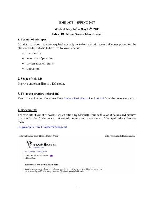
4. Background
The web site ‘How stuff works’ has an article by Marshall Brain with a lot of details and pictures
that should clarify the concept of electric motors and show some of the applications that use
them.
(begin article from Howstuffworks.com)
1

disassembly sequence
4

(end article from Howstuffworks.com)
Your objective in this lab is to identify the parameters (Ra, La, km, K, τelectrical, τoverall) of a DC
motor using step response testing.
The motor is represented by the following model (Figure 1):
ea(t)
Ra
La
T(t)=kmia(t)
Figure 1: Electromechanical model of a DC motor
The labeled items are
ea(t) = input voltage
Ra = resistance
La = inductance
ia(t) = current
eb(t) = back emf
T(t) = torque
ω(t) = shaft angular velocity
J = moment of inertia
b = viscous damping coefficient
km = torque constant
7
ω(t)
ia(t) eb(t)= kmω(t)
J
b

Equations
We start with two equations, one electrical and the other mechanical. Summing the loop voltages
gives:
dia
(t)
(1) La + R ai
a (t) = ea
(t) − eb
(t)
dt
Summing the torques present at the motor’s output shaft gives
(2) J ω&
(t) + bω(
t)
= T(t)
Equations (1) and (2) are two first-order ODE’s. They are related by the motor’s torque-current
relationship and by the back-emf produced by the motor rotation:
(3) T(t) = kmia(t)
(4) eb(t) = kmω(t)
Note that the same constant (km) appears in both equations (3) and (4). This is only true if we use
SI units. Two constants (called the motor torque constant and the back-emf (electromotive force)
coefficient) are required when English units are used.
The motor’s time response has two time constants (τ) – we’ll call these an electrical and a
mechanical time constant. The electrical time constant is almost always a lot faster than the
mechanical time constant, and is often neglected in modeling the motor dynamics. This is called a
dominant-pole approximation, and is a useful approach to simplifying the model.
To test this assumption, the electrical time constant can be measured by locking the motor shaft in
place. Then eb = kmω(t) = 0, and equation (1) simplifies to:
dia
(t)
(5) La + R ai
a (t) = ea
(t)
dt
If we apply a voltage step to the motor (ea(t) = ea for t > 0), we expect to see an exponential
La
ea
response with a time constant given by τ = and a steady-state current of i ss = . We can
R a
R a
use measurements of τ and iss to determine Ra and La.
When the motor shaft is unlocked, we can use steady-state measurements of the input current,
motor speed, and applied voltage to determine the torque constant (km) and the viscous damping
coefficient (b). In steady-state, all the derivative terms in equations (1) and (2) are zero, so we
have:
(6) k mωss
= ea
− R ai
a, ss
k mi
a, ss
(7) ωss
=
b
The final parameter to be measured is the motor’s moment of inertia, J. If the electrical time
constant is very fast, the dynamic model for the motor is simplified by neglecting the first term in
equation (1):
(8) i (t) =
e (t) − e (t)
R a a a b
8

Then we can find the motor torque by substituting equations (3) and (4) into equation (8):
2
k m k m
(9) T()
t = ea
() t − ω()
t
R a R a
Finally, if we substitute equation (7) into equation (2), we have the following relationship
between the motor speed and the input voltage:
2
b + k m k m
(10) Jω& () t + ω()
t = ea
() t
R a R a
As a result, if we apply a voltage step to the motor (ea(t) = ea for t > 0), we expect to see an
exponential response with a time constant given by:
(11)
5. Motor and Power Amplifier Overview
b + k
τ =
JR
Since the ELVIS prototyping board cannot output enough current to drive the motor, the power
amplifier is used to buffer your output voltage. The power amplifier has a gain of approximately
2 V/V, so if the input voltage is 1 V, the output from the power amplifier is 2V. The power
amplifier has a current sensor which can be used to measure the current applied to the motor. The
current sensor output can be measured at the red test point (labeled VCURR+). The current
sensor has a gain of 2 V/A, so if the voltage measured at VCURR+ is 1V, the output current is
500 mA.
The motor contains a tachometer (literally, ‘measurement of speed’). The angular speed is
computed from the tachometer’s RMS voltage output using the following relationship:
(12) ω [rad/sec] = 52.4 [Volts RMS]
6. Procedure
A. Measure the motor’s electrical characteristics
In this part of the lab, you will measure the motor’s electrical time constant to determine the
armature inductance La.
1. First, use the DMM to measure the armature resistance, Ra. Insert two test leads with minihook
or alligator-clip ends into the DMM front panel on the current side (not the voltage
side). Attach the test leads to the motor input wires. Set the DMM for resistance
measurements by selecting the Ω key. Make multiple measurements (>4) at different motor
shaft angles. Average the values and record this as Ra below. Since this is a low resistance,
the ELVIS DMM isn’t particularly accurate. You will compute the resistance again below.
2. Now, turn off the power to your prototyping board and make sure that the power amplifier is
plugged in and turned off. Make the electrical connections shown in Figure 2 below. Connect
the BNC1 connector on the ELVIS breadboard to the input of the power amplifier with a
BNC cable. Connect the motor input wires to the screw terminals on the output side of the
power amplifier. Next, connect the current sensor using mini-hook test leads connected to
9
a
2
m

Banana C and D on the breadboard. Attach the mini-hooks to the VCURR+ and AGND test
points on the Power Amplifier. Finally, connect the tachometer to Banana A and B using
banana leads.
3. Make the following jumpers on the Elvis prototyping board:
• DAC0→BNC1+ GND→BNC1-
• DAC1→Oscilloscope - Trigger
• Banana A→ACH0+ Banana B→ACH0-
• Banana C→ACH1+ Banana D→ACH1-
Current Sensor
Tachometer
Elvis
BNC 1
Banana C
Banana D
Banana A
Banana B
BNC Cable
Banana Leads
VIN
Test Points
VCURR
AGND
Figure 2: Electrical connections.
4. Lock the motor shaft so that you can measure the electrical time constant. Use the screw
provided to lock the shaft in place.
5. Create test and triggering waveforms as illustrated below using the Waveform Editor. The
triggering waveform will be used to trigger the oscilloscope slightly before the rising-edge on
the test waveform, which will be applied to the motor through the power amplifier. The test
waveform amplitude is 0.5 V in order to produce a 1 V output from the power amplifier.
Triggering waveform, 5V amplitude
1 s
a. Open the Arbitrary Waveform Generator SFP in ELVIS, then select the Waveform Editor
key and make the following settings on the Waveform Editor:
• Units: Hz
• Sample Rate: 10000.0
• Segment duration to 2 sec.
b. First create a test waveform that has peak amplitude of 0.5V. Select the New Component
key to add a component. Make the following settings for this component:
• Function Library: Square.
• Amplitude: 0.25 V
• Offset: 0.25 V
10
Power Amplifier
Banana Leads
Screw Terminals
VOUT
AGND
Test waveform, 0.2V amplitude
t
Motor
Wires
DC
Motor
Jacks
Red
Black

• Frequency (Hz): 0.5
c. Click on FILE>>Save As and save the waveform to a waveform data file (.wdt format).
d. Repeat for a triggering waveform. Select the New Component key to add a component.
Make the following settings for this component:
• Function Library: Square
• Amplitude: 2.5 V
• Offset: 2.5 V
• Frequency (Hz): 0.5
• Phase: 4.0
• Duty Cycle (%): 1.0000
e. Click on FILE>>Save As and save the waveform to a waveform data file (.wdt format).
6. You will run three tests of the motor response using input amplitudes of 3V, 4V, and 5V. In
the Arbitrary Waveform Generator SFP adjust the update rate to be 10,000 S/s. Load the test
waveform into DAC0 and adjust the Gain to 3. Load the trigger waveform into DAC1. Press
the Play All soft key.
7. Turn on the Prototyping Board Power and the power amplifier.
8. Start Oscilloscope SFP. Set the source for channel A to ACH1. Select the Display ON
softkey. Adjust the timebase to 2 ms/div and set the Vertical Scale to 200 mV/div. Set the
trigger source to TRIGGER and the slope to descending.
9. Press the single key and press the log key. Save the data as (.txt).
10. Press the Stop All soft key in the Arbitrary Waveform Generator, increase the gain to 4 and
press the play all key then repeat step 11. Adjust the gain to 5 and repeat.
11. Open the 3 files in excel. Convert the current sensor voltage into current in Amperes. Plot the
current versus time for the three input voltages on the same plot. Make sure to label your
axes. Hand in the plot with your lab write-up.
12. Compute the 63% rise time (τ) and the steady-state current for each plot and record them in
the table below. Calculate the armature resistance (Ra) from the steady-state current and the
input voltage. Average for the three voltages. Given that τ = La/Ra compute La and average
for the 3 voltages.
B. Determine the system time constant τ
In this part of the lab you will measure the system time constant and use it to calculate the
motor’s moment of inertia.
1. Remove the screw and allow the output shaft to rotate freely.
2. Now, you will test the motor time response with three input amplitudes: 4V, 5V, and 6V. Set
the DAC0 gain in the Arbitrary Waveform Generator to 4 and press play.
3. View the Oscilloscope SFP in ELVIS. Set the source for channel A to ACH0. Adjust the
timebase to 200 ms/div and set the Vertical Scale to 1 V/div.
4. Press the Single key and press the Log key. Save the data as (.txt).
11

5. Repeat for gains of 5 and 6.
6. Download and open the file AnalyzeTachoData.vi from the course website. Input the sample
period for your data the dt control. If you’re not sure what this is, you can open any of your
.txt files and read the dt value in Excel.
7. Run this vi and open one of your data files. It will then ask you to input a name to save the
data. The data saved is after the input data has been rectified and filtered. You will see two
waveform graphs. The first one shows the data exactly as it was read in. The second one is the
rectified and filtered data.
8. Experiment with the filter block in the VI. The default filter is a 3 rd -order butterworth filter
with a 25 Hz cutoff frequency. Try adjusting cutoff frequency to a lower and higher
frequency. What do you observe? Next, try changing the filter order. Does this have any
effect on your result?
9. Open the filtered data in Excel. Plot all three on the same graph, determine the 63% rise times
and record the values in the table below. Make sure to label the axis and hand in the plots
with your lab write up.
C. Create a VI to make steady-state measurements of current & motor speed vs voltage
In this part of the lab you will write a VI based on the VI from Lab 2 (lab2.vi) to automatically
measure the steady-state speed and input current of the motor as the input voltage is increased.
This time, instead of graphing the results you will store the RMS tachometer voltage and the
mean input current to a file for later analysis.
1. Open your VI from Lab 2 or use the file downloaded from the class web site. Save it under a
new file name. A picture of the changes that you will make to the block diagram is shown in
Figure 3.
input voltage
Figure 3: Wiring the DAQ Assistant to the Write LVM File VI.
2. Go to the block diagram and delete the XY graph, the Build XY Graph and the two To
DDT vi’s. In their place, create a block to store the data to a Labview measurement (LVM)
file. Go to Functions»Output and place a Write LVM block outside the While Loop. Select
Save to one file and check Ask user to choose file. Under X Values Column select One
Column Only. Leave the default settings for all the other values.
12

3. Place a Merge Signals block next to the data input on the Write LVM from
Functions»Signal Manipulation. Use the mouse to resize the block to give it three inputs.
This will allow you to store three columns of data in the file (the input voltage, the mean
current input, and the RMS tachometer reading).
4. Change the Time Delay in the second frame of the stacked sequence. Use a delay that is at
least 3τ so that the motor will have reached a steady speed before you make any
measurements.
5. Modify the DAQ Assistant Express VI in the third sequence frame to measure 250 samples of
the tachometer and current sensor outputs. To do this, make the following configurations in
the DAQ Assistant configuration wizard:
• In addition to measuring the voltage on ai0 (ACH0), add a new voltage measurement
to measure ai1 (ACH1).
• In the Task Timing section, select N Samples.
• Set the Samples to Read to 250, and set the sample rate to 5000 samples/sec.
6. The DAQ Assistant you created will produce 250 samples per channel with each iteration. We
will first convert the data into two arrays with 250 samples each. Go back to the block
diagram, right click and select Functions»Signal Manipulation and choose From DDT.
Place this in the while loop and select 2D array of scalars – columns are channels then
click ok. Wire the output of the DAQ Assistant to the input of the From DDT. Add an Index
Array block and split the 2D array into two 1D columns as was done in Lab 3.
7. We will store only the RMS value of the tachometer output and the mean value of the current
sensor output. Right click and select the RMS block from the menu: Functions»All
Functions»Analyze»Mathematics»Prob and Stat. Place this in the while loop and wire the
first data array (from ACH0) to the RMS block. Repeat the process to create a Mean block
and wire it to the second data array (from ACH1).
8. Wire the output voltage (which used to be connected to the X-axis of the XY graph) to the top
terminal on the Merge Signals block. Wire the output of the Mean block and the RMS block
to the border of the While loop. Right click on the two new loop tunnels at the border of the
While loop and select “Enable Indexing.” Wire these loop tunnels to the second and third
inputs to the Merge Signals block. Labview will automatically create To DDT blocks to
convert the signals to Dynamic Data Type.
9. Save your completed VI.
Testing
1. Make the following front panel settings of the VI: Vmin = 1.5 V, Vmax = 3.25 V, Nsteps = 7.
2. Press the Run key. When your program is complete, you will be prompted to save your data
to a file.
3. Open the file with Excel and check the data. Your current sensor and tachometer readings at
Vin = 0.4V, 0.5V and 0.6V should agree with the steady-state values from Part B. If they do
not, there probably something wrong with your VI. Ask your TA for help.
13

4. In the Excel spreadsheet, make three new columns to convert your measured data into the
armature voltage (ea), the steady-state current (ia,ss) and motor speed (ωss) using the
conversion factors for the power amplifier (5 V/V), the current sensor (2 V/A) and the
tachometer (52.4 rad/sec/V).
5. Make a plot with ωss on the y-axis and ia,ss on the x-axis. Using eq. (7), the slope of this line is
equal to (km/b). Find the slope, label the axes of this plot and save it to hand in with your
report.
6. Create an additional column to compute (ea - Ra ia,ss). Make a second plot with ωss on the xaxis
and ea - Ra ia,ss on the y-axis. Using eq. (6), the slope of this line is equal to km. Find the
slope, label the axes of this plot and save it to hand in with your report.
7. Write-up
In your typed lab report, indicate the following information by including tables such as those
shown below.
A. Electrical Characteristics
Ra = ________Ω Measured
Power Amp
Output, ea
[V]
3
4
5
Armature
Current,
ia,ss [mA]
Average:
B. Determining System Time Constant
14
Ra
[Ω]
Step Input (V) τ
4
5
6
Average
τ
[ms]
La
[mH]
Compare the electrical time constant to that of the overall system. Is it a good assumption to
neglect the electrical time constant?

C. Measuring the Motor Steady State Response
Attach the two plots for ia,ss vs. ωss and for ωss vs. (ea - Ra ia,ss). Use the slopes of these lines to
calculate:
km [N-m/A] = _______
b [N-m/(rad/sec)] = ________
Use your measurements of τ, km, Ra and b to calculate the motor inertia from eq. (11):
J [kg-m 2 ] = ________
Use your measurements of km, Ra, and ωss to calculate the maximum value of Torque from eq.
(9):
T [N-m] = _________
Finally calculate the horsepower of your motor.
H [horsepower] = 0.05294 T[N-m] ωss[rad/s]
H = _________
15