A Simplified Eigenstrain Approach - Department of Mechanical and ...

A Simplified Eigenstrain Approach for Determination
of Sub-surface Triaxial Residual Stress in Welds
Michael R. Hill
Mechanical and Aeronautical Engineering Department
University of California, Davis
Email: mrhill@ucdavis.edu
Drew V. Nelson
Mechanical Engineering Department
Stanford University
Email: dnelson@leland.stanford.edu
Abstract
This paper discusses the localized eigenstrain method, a new technique for the determination of
triaxial residual stresses deep within long welded joints. The technique follows from the “Inherent
Strain Method” developed by Ueda, which uses a combined experimental and analytical approach
to determine the source of residual stress (i.e., “eigenstrain” or, equivalently, “inherent strain”) by
sectioning and strain measurement. Once the eigenstrain field is found, it is used to deduce
residual stress in the original body prior to sectioning. The main advantage of this method is that
residual stress is estimated within the entire welded joint. On the other hand, the localized
technique focuses on finding residual stress only in the bead region of the joint, often a critical
region with respect to fracture and fatigue. Because the method focuses only on near-bead
residual stress, the required experimental effort is greatly reduced in comparison with Ueda’s
original formulation. In the paper, we begin by presenting the eigenstrain method in general and
then describe localization of the technique. A model problem is then developed and used to
investigate the accuracy of the technique through numerical modeling. Finally, the advantages and
drawbacks of this new method are discussed.
Nomenclature
ε*
ε* ij
σ
σ ij
ε ˜ *
σ ˜
eigenstrain tensor
individual component of eigenstrain
stress tensor
individual component of stress
assembled vector of eigenstrain
interpolation parameters
assembled vector of stress changes
1 Introduction
M linear system relating stress to
˜
eigenstrain
W, T, D width, thickness, and depth of
welded sample
B size of the region of interest
ξ non-dimensional measure within the
chunk geometry
Ueda has proposed a general method for determining triaxial residual stress, the “Inherent Strain
Method” (Ueda, 1975). A distinctive characteristic of this class of procedures is that residual
stress is found through estimation of the source of residual stress within an object. Experts on
continuum mechanics and elasticity, including Timoshenko and Goodier (1970) and Mura
(1987), acknowledge that residual stress is the result of some inelastic strain field which does not
satisfy compatibility. This strain field is present due to mechanical and thermal processes which
the body has undergone. Ueda refers to the inelastic, non-compatible strain as “inherent strain”,
while we will adopt Mura’s terminology, by calling it “eigenstrain”. For a welded joint, the
1

2
eigenstrain field is the combination of thermal, transformation, and plastic strains which are the
net result of the welding process.
Although residual stress is caused by eigenstrain, it is also a function of the geometry of the
body in which it is imposed. For example, imagine a long welded plate. If a sample is removed
from the plate that is short along the weld-length, stress will be released in removing the sample.
The stress has changed, but the eigenstrain within the removed sample remains the same,
assuming that the cutting process results only in elastic deformation of the sample. The
eigenstrain method is a form of destructive sectioning, as strain released during geometry
changes is used to deduce the underlying eigenstrain distribution. The eigenstrain distribution is
complicated, however, since it represents the spatial variation of a tensor quantity. If the
eigenstrain can be found, it can then be used to estimate residual stress in the original sample,
prior to cutting, and also in the structure from which the sample was removed.
Application of the eigenstrain approach to residual stress in continuously welded joints was
presented by Ueda, et al. (1985) and further studied in a recent paper (Hill and Nelson, 1995).
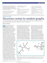
Consider a long, continuously welded plate with directions which correspond to the weld bead as
shown in Figure 1. These consist of the transverse, perpendicular, and longitudinal directions
relative to the direction of welding. We have chosen corresponding coordinates x,
y,
and z,
respectively. The assumption of continuous welding allows consideration of an eigenstrain field
that is dependent on the transverse and perpendicular coordinates, while independent of the
longitudinal coordinate. The basis for this assumption is that each plane in the weld
cross-section, like the two shaded in Figure 2, is thought to experience the same thermal and
mechanical processes during a continuous weld pass. This assumption holds neither in the
thermal nor the mechanical sense near the ends of the joint, but the assumption may be
reasonable in the remainder of the joint, as indicated by experimental evidence presented by Hill
and Nelson (1996).
Long. (z)
Perp. (y)
Trans. (x)
Figure 1 – Directions relative to a weld.
Long. (z)
Perp. (y)
Trans. (x)
Figure 2 – Two planes which have the same
eigenstrain distribution.
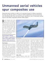
An illustration of Ueda’s technique is shown in Figure 3. A sample of welded plate, obtained
from the structure of interest, is instrumented with an array of strain gages on one of its faces
normal to the z-axis
(shaded in the figure). Two strain-relaxation measurements are then
performed, one from block to thin slice and the other from slice to small pieces (dice), each
containing a strain gage. Since the slice is in plane stress, slice-to-dice data allow determination
of the x-y distribution of the eigenstrain components in the transverse-perpendicular plane ( ε* xx ,
ε* yy , and ε* xy ). Using these results with the block-to-slice relaxation data allows determination
of the eigenstrain component associated with the longitudinal direction ( ε* zz ). The two
additional components of eigenstrain ( ε* yz and ε* zx
) are assumed to be zero because they
would cause asymmetrical stresses to arise in the welded joint which is contrary to empirical
observation (Ueda, et al., 1985). Ueda’s method, then, allows determination of the x-y

distribution of the entire eigenstrain tensor and assumes the distribution is independent of z.
Since the total eigenstrain field is known, residual stress can be found in the original specimen
geometry, prior to sectioning, or in the structural geometry prior to specimen removal by
imposing the eigenstrain field in an elastic finite element model (Hill, 1995).
The determination of eigenstrain components from measured changes in strain involves
solution of a linear system found by repetitive finite element method calculations, as described
by Hill and Nelson (1995). For a given sectioning operation, the linear system relates measured
changes in stress at specific points on the object to parameters of an eigenstrain interpolation.
This linear system is very much like the stiffness matrix of finite element analysis (FEA) which
relates internal forces to internal displacements. Just as in FEA, the formulation of the linear
system depends on the type of interpolation chosen (i.e., the "shape functions") and the
organization of the interpolation parameters (i.e., "assembly"). In all of the work reported here,
we choose to approximate the distribution of each component of eigenstrain using linear
interpolation in spatial coordinates. Once the interpolation scheme and an arbitrary system
organization (row and column order) are adopted, a linear system can be formed relating stress to
eigenstrain,
σ = M ⋅ ε* . [1]
˜ ˜ ˜
Given measured stress components, σ , the eigenstrain parameters, ε* (akin to nodal values of
˜
˜
displacement in FEA) can be found by inversion of Equation [1].
Long. (z)
Figure 3 – Pictorial representation of the
slice-and-dice method proposed by Ueda (1985).
Perp. (y)
Trans. (x)
Figure 4 – Region in a welded block where
residual stress is determined by the localized
eigenstrain method.
A major drawback of Ueda’s method is that a daunting number of strain-relaxation
measurements must be conducted using sectioning and strain gage instrumentation. Recently, the
authors have developed a localization of Ueda’s approach which allows stress to be determined
only in close proximity to the weld bead (Hill, 1996b). Limitation to this region is reasonable
from the standpoint of failure assessment, as weld defects and large residual stresses are likely to
exist together only in or very near the weld bead. Since the transverse extent of the weld bead is
often on the order of the thickness of the welded plate, the localized technique was developed to
find residual stress within the hexahedral region shaded in Figure 4.
2 Description of the Localized Eigenstrain Method
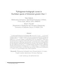
Localization of the eigenstrain method for a continuous weld is based on a modification of the
sectioning technique proposed by Ueda and is shown schematically in Figure 5. This process
differs from that shown in Figure 3 in two ways. First, only the bead region on the face of the
welded sample, shown shaded in the figure, is instrumented with strain gages. Secondly, the
sectioning process includes an intermediate “chunk” geometry between slice and dice, created by
3

4
removing the region of interest from the slice. This modified sectioning process allows for
separation of the eigenstrain field into two portions, one lying inside and one outside of the
region of interest.
Figure 5 – Pictorial representation of the localized
eigenstrain technique for continuous welds.
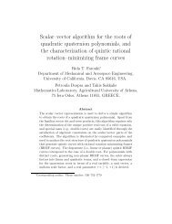
The localized eigenstrain method is most easily described with a specific geometry,
sectioning plan, and strain measurement scheme in mind. Assume that a block of material has
been removed from a welded joint and has dimensions shown in Figure 6(a). A region of interest
in the xy-plane
of this block is identified, shown shaded in the figure. The free surface of this
region is instrumented as shown in Figure 7. Following instrumentation, the block is sectioned as
shown schematically in Figure 5 with dimensions of the slice and chunk shown in Figure 6(b)
and (c). Strain changes are measured that accompany removal of the slice from the block,
removal of the chunk from the slice, and finally cutting the slice into dice. Assuming that the dice
are small enough relative to the spatial gradients of eigenstrain, the dice will be stress-free. Using
relaxation data with elastic stress-strain relations for plane stress, residual stress can then be
computed at the free-surface measurement sites on the block, slice, and chunk geometries. The
localized eigenstrain method then uses these reduced stress data to estimate the eigenstrain
distribution which, in turn, allows stress to be computed at any point in the region of interest.
2.1 Division of eigenstrain into
ε*
A and ε*
B
Figure 6 – (a) Block of material removed from a
welded joint, (b) slice removed from the block, and
(c) chunk removed from the slice. The chunk would
further be sectioned into dice.
One of the crucial steps in assuring success of the localized eigenstrain method is separation
of the eigenstrain into two parts. The first part, ε* B , is found from stress in the chunk, and the
second part, ε* A , from stress in the slice. This second part of the eigenstrain is further divided
into two distinct parts. The first is eigenstrain which lies within the region of the chunk, but does
not cause stress once the chunk is cut free from the slice. The second part of ε* A
is an
approximate representation for eigenstrain which lies outside of the chunk region. To correctly
account for this division, the x-interpolation
for each portion of the eigenstrain has been carefully
developed (Hill, 1996b). The y-interpolation,
on the other hand, is a simple linear interpolation
with seven equally spaced nodes.
T
z
W = 203mm
T = 38mm
D = 127mm
B = 0.8T
y
x
B
W
T
3B
B
D/20
D
D/20
(a)
(b)
(c)

y = 0
-1/6 T
-1/3 T
-1/2 T
-2/3 T
-5/6 T
-T
x o–
1/3 B
x = xo
Region of
Interest
x o+
1/3 B
= Strain Measurement Location
Figure 7 – Measurement locations within the
region of interest where three-element strain gage
rosettes would be placed.
2.2 Scheme for interpolation of
ε* B
ε*
B
Functions used to interpolate in the x-direction
are shown in Figure 8. These functions
are the result of two important considerations. First, eigenstrain distributions which would cause
stress-free deformation in the chunk are explicitly excluded by proper choice of the interpolation
scheme. For each particular component of eigenstrain, this amounts to assuring that the
compatibility relations of elasticity cannot be satisfied by any combination of the interpolation
functions. Second, spacing between interpolation nodes for a particular component is constant. It
was found that even spacing produces a linear system for eigenstrain determination which is as
well conditioned as possible, and therefore produces superior estimates of the eigenstrain
parameters. The functions shown in Figure 8 satisfy these two criteria.
2.3 Scheme for interpolation of
ε*
A
ξ=−0.5 ξ=0
ξ=0.5
ξ=−0.25 ξ=0.25
ξ=−1/6 ξ=1/6
(a) Interpolation of ε* xx
(b) Interpolation of ε* yy
(c) Interpolation of ε* xy
Figure 8 – Interpolation functions used to distribute
ε* B in the chunk. ξ = ( x – xo) ⁄ B , where xo
is the
center of the chunk and B is the width of the region
of interest. Measurements taken at ξ = -1/3, 0, 1/3.
Again, there are two parts of the eigenstrain distribution which cause stresses in the slice and
cannot be predicted by stresses in the chunk. The first part is the eigenstrain which causes stress
when present in the chunk region of the slice geometry, but causes no stress once the chunk is cut
free. The interpolation of this portion of ε* A varies for each component of eigenstrain, as shown
in Figure 9(a) and (b). For ε* xx , there are no stress-free modes of eigenstrain distribution which
are not also stress-free in the slice. The second part of the eigenstrain to be determined by stress
in the slice is the eigenstrain which lies outside of the chunk region, . It was found, by trial
ξ=−5/6 ξ=−0.5 ξ=0.5 ξ=5/6
ξ=−5/6 ξ=−0.5 ξ=0.5 ξ=5/6
ξ=−5/6 ξ=−0.5 ξ=0
ξ=0.5 ξ=5/6
ε* A
(a) Interpolation of ε* yy
(b) Interpolation of ε* xy
(c) Sawtooth functions common
to all components.
Figure 9 – Interpolation functions used to distribute eigenstrain determined from
stress in the slice, ε* A . ξ = ( x – xo) ⁄ B , where xo is the center of the chunk.
5

6
and error, that the specific functions used to interpolate this part of the eigenstrain does not alter
the results of the stress approximation within the region of interest.
Therefore, the simple
sawtooth functions shown in Figure 9(c) are used to interpolate each component of eigenstrain
outside the region of interest.
2.4 Interpolation for longitudinal eigenstrain, ε* zz
In estimating the longitudinal eigenstrain component, there is no distinction between the
chunk and the slice, except in a discontinuity in interpolation across the boundary of the region of
interest. That is, the solution procedure for finding a parameterized distribution of ε* zz is the
same as in the non-localized method, except for the interpolation functions used. The proper
interpolation for ε* zz is the same as that used for ε* xx as shown in Figure 8(a) and Figure 9(c).
To find the longitudinal eigenstrain, the distribution of the planar components of eigenstrain
is estimated as described above, then these are imposed in a finite element model of the block to
find the stresses that they cause on its free-surface. These stresses are subtracted from the
experimental estimates of residual stress on the block free-surface, and the differences used to
determine the parameters in the interpolation.
3 Numerical Simulation of the Method
The accuracy of the method described above will depend greatly on the residual stress
distribution being measured. Our goal in this section is to assess the accuracy with respect to one
residual stress system in particular through numerical simulation of the technique.
The goal of the simulation is to find residual stress within the sample of welded plate
depicted in Figure 6(a). Residual stress is produced in a finite element model of each specimen
shown in Figure 6 by introduction of an eigenstrain field. The resulting residual stress state is
fully three-dimensional, and exists everywhere within the body. The specific eigenstrain field
used is given in detail in an earlier paper (Hill and Nelson, 1995). This field was developed to
produce a complicated residual stress state that resembles the character of thick-weld residual
stress; however, this field should not be construed to be the residual stress state present in any
real weld. Its sole purpose is to provide a basis by which to compare techniques for residual
stress determination. Residual stresses on specific contours through the weld are shown in
Figures 10 and 11. These stresses are the result of a direct finite element computation and are
identified as “exact,” meaning that a perfect measuring technique would obtain the same results.
The linear systems are formed for determination of ε* B , ε* A , and ε* zz using the
interpolation schemes described above. These systems are then used with stress on the
free-surfaces of the chunk, slice, and block computed by FEA. That is, the FEA results on the
free-surface are used as input to the localized eigenstrain method. Parameters determined from
solution of these systems are then used to interpolate the total eigenstrain on a model of the block
geometry, and residual stress estimates within the block are obtained. Stress estimates at the weld
midlength are compared to FEA results in Figure 12. Good agreement between the two sets of
results is obtained. The largest errors present are in near the surface of the joint.
4 Discussion
ε* zz
Numerical simulation indicates that the localized eigenstrain method can be used to estimate
residual stresses at the midplane of the block to a good degree of accuracy. The maximum
difference between estimated and exact stress is smaller than that obtained using the
σ zz

Figure 10 – Residual stresses at the center of the
sample, through the thickness of the plate.
Stress (MPa)
Stress (MPa)
Long. (z)
150
100
50
Stress (MPa)
0
-50
-100
250
200
150
100
50
0
-50
-100
-150
Perp. (y)
200
150
100
50
0
-50
-100
-150
-38
Trans. (x)
-28.5
FEA: σ xx
FEA: σ yy
FEA: σ zz
FEA: σ xy
Exact: σ xx
Exact: σ yy
Exact: σ zz
-19 -9.5
y (mm)
-35 -30 -25 -20 -15 -10 -5 0
FEA: σ xx
FEA: σ yy
FEA: σ zz
FEA: σ xy
y (mm)
0
Long. (z)
Perp. (y)
Trans. (x)
-50
0 50.75 101.5
Figure 11 – Residual stress at the center of the
weld length, across the top surface.
Figure 12 – (a), (b), (c): Stress at the midplane of the block induced by the model eigenstrain
function as computed by FEA, compared to those estimated by the localized eigenstrain
method. Each plot is for a different x-location, as indicated at the bottom-right.
(d) Error in mid-plane stress estimates for the localized eigenstrain technique and the "regular" technique
proposed by Ueda (adapted from (Hill and Nelson, 1995)) on the line x = 96.5mm.
Stress (MPa)
(a) (b)
-35 -30 -25 -20 -15 -10 -5 0
y (mm)
(c)
Loc. ε*: σ xx
Loc. ε*: σ yy
Loc. ε*: σ zz
Loc. ε*: σ xy
Midplane, and x=86.4
Loc. ε*: σ xx
Loc. ε*: σ yy
Loc. ε*: σ zz
Loc. ε*: σ xy
Midplane, and x=107
Stress (MPa)
Stress (MPa)
250
200
150
100
50
0
-50
-100
-150
30
20
10
0
-10
-20
-30
-40
200
150
100
50
0
FEA: σ xx
FEA: σ yy
FEA: σ zz
FEA: σ xy
Loc. ε*: Error σ xx
Loc. ε*: Error σ yy
Loc. ε*: Error σ zz
x (mm)
(d)
Exact: σ xx
Exact: σ zz
152.2 203
-35 -30 -25 -20 -15 -10 -5 0
y (mm)
Reg. ε*: Error σ xx
Reg. ε*: Error σ yy
Reg. ε*: Error σ zz
-35 -30 -25 -20 -15 -10 -5 0
y (mm)
Loc. ε*: σ xx
Loc. ε*: σ yy
Loc. ε*: σ zz
Loc. ε*: σ xy
Midplane, and x=96.5
Midplane, and x=96.5
7

8
“non-localized” eigenstrain method, as shown in Figure 12(d). The improved accuracy is the
result of the improved shape functions used to interpolate the eigenstrain. In developing these
functions, an effort was made to minimize the number of eigenstrain components which are lost
to modes of stress-free deformation during the inversion of Equation [1]. Overall, the difference
between estimated and exact stress for either method is fairly small in relation to the levels of
stress present in the block, as shown in Figure 12(a)–(c).
The development of the localized eigenstrain technique adds to the ability of the technique
developed by Ueda. The localized method has the advantages of Ueda’s method, while being
easier to implement for determination of stresses near a weld bead. The experimental effort
required for the two techniques differs greatly. Implementation of Ueda’s technique, as described
by Hill and Nelson (1995), would require 140 three-element strain gage rosettes. The localized
technique, on the other hand, would require only 21. This is a large reduction in effort, which
makes use of the eigenstrain technique much more practical. Not only is the experimental effort
reduced, but the computational burden as well since one finite element solution must be obtained
for each eigenstrain parameter in the interpolation system. As described by Hill and Nelson
(1995), Ueda’s technique had 500 such parameters while the method presented here has only
147. For these reasons, the localized eigenstrain method adds ease of execution to the previously
existing method developed by Ueda.
5 Conclusion
A localized version of Ueda’s inherent strain (or, eigenstrain) method has been developed to
enable determination of weld residual stresses by sectioning with a considerable reduction in
experimental and computational efforts required. The new method retains the ability of the
eigenstrain approach to estimate triaxial residual stress through the thickness of the welded joint
but obtains results only in the bead region.
6 References
Hill, M. R. and D. V. Nelson (1995). “The inherent strain method for residual stress determination
and its application to a long welded joint.” PVP v. 318. New York, NY, ASME. pp. 343-352.
Hill, M. R. and D. V. Nelson (1996). “Determining residual stress through the thickness of a
welded plate.” PVP v. 327. New York, NY, ASME. pp. 29-36.
Hill, M. R. (1996b). Determination of Residual Stress Based on the Estimation of Eigenstrain,
PhD Dissertation, Stanford University.
Mura, T. (1987). Micromechanics of Defects in Solids. Dordrecht, Netherlands, M. Nijhoff.
Timoshenko, S.P. and J.N. Goodier, 1970, Theory of Elasticity. New York, McGraw-Hill.
Ueda, Y., K. Fukuda, et al. (1975). “A new measuring method of residual stresses with the aid of
finite element method and reliability of estimated values.” Transactions of the JWRI 4(2): pp.
123-131.
Ueda, Y., Y. C. Kim, et al. (1985). “Measuring Theory of Three-Dimensional Residual Stresses
Using a Thinly Sliced Plate Perpendicular to Welded Line.” Transactions of the JWRI 14(2):
pp. 151-157.