Torsion

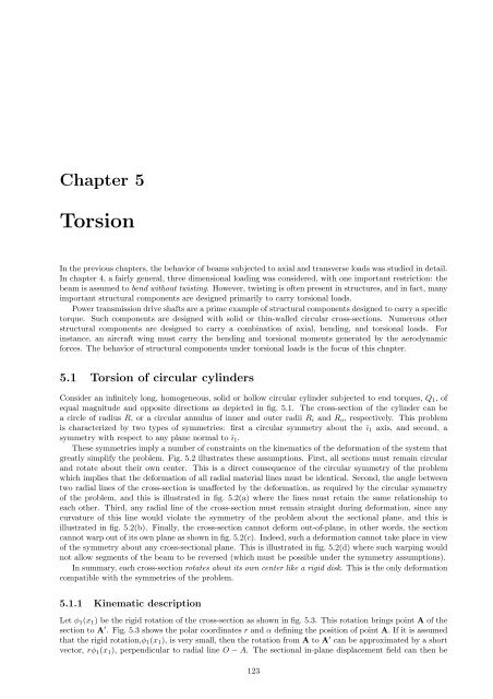
Chapter 5
Torsion
In the previous chapters, the behavior of beams subjected to axial and transverse loads was studied in detail.
In chapter 4, a fairly general, three dimensional loading was considered, with one important restriction: the
beam is assumed to bend without twisting. However, twisting is often present in structures, and in fact, many
important structural components are designed primarily to carry torsional loads.
Power transmission drive shafts are a prime example of structural components designed to carry a specific
torque. Such components are designed with solid or thin-walled circular cross-sections. Numerous other
structural components are designed to carry a combination of axial, bending, and torsional loads. For
instance, an aircraft wing must carry the bending and torsional moments generated by the aerodynamic
forces. The behavior of structural components under torsional loads is the focus of this chapter.
5.1 Torsion of circular cylinders
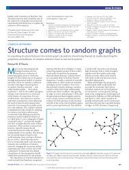
Consider an infinitely long, homogeneous, solid or hollow circular cylinder subjected to end torques, Q1, of
equal magnitude and opposite directions as depicted in fig. 5.1. The cross-section of the cylinder can be
a circle of radius R, or a circular annulus of inner and outer radii Ri and Ro, respectively. This problem
is characterized by two types of symmetries: first a circular symmetry about the ī1 axis, and second, a
symmetry with respect to any plane normal to ī1.
These symmetries imply a number of constraints on the kinematics of the deformation of the system that
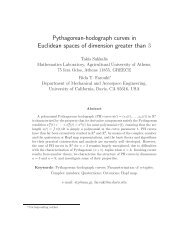
greatly simplify the problem. Fig. 5.2 illustrates these assumptions. First, all sections must remain circular
and rotate about their own center. This is a direct consequence of the circular symmetry of the problem
which implies that the deformation of all radial material lines must be identical. Second, the angle between
two radial lines of the cross-section is unaffected by the deformation, as required by the circular symmetry
of the problem, and this is illustrated in fig. 5.2(a) where the lines must retain the same relationship to
each other. Third, any radial line of the cross-section must remain straight during deformation, since any
curvature of this line would violate the symmetry of the problem about the sectional plane, and this is
illustrated in fig. 5.2(b). Finally, the cross-section cannot deform out-of-plane, in other words, the section
cannot warp out of its own plane as shown in fig. 5.2(c). Indeed, such a deformation cannot take place in view
of the symmetry about any cross-sectional plane. This is illustrated in fig. 5.2(d) where such warping would
not allow segments of the beam to be reversed (which must be possible under the symmetry assumptions).
In summary, each cross-section rotates about its own center like a rigid disk. This is the only deformation
compatible with the symmetries of the problem.
5.1.1 Kinematic description
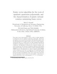
Let φ1(x1) be the rigid rotation of the cross-section as shown in fig. 5.3. This rotation brings point A of the
section to A ′ . Fig. 5.3 shows the polar coordinates r and α defining the position of point A. If it is assumed
that the rigid rotation,φ1(x1), is very small, then the rotation from A to A ′ can be approximated by a short
vector, rφ1(x1), perpendicular to radial line O − A. The sectional in-plane displacement field can then be
123

124 CHAPTER 5. TORSION
Q 1
i 3
R
i 2
i 3
Circular
cylinder
i 2
R i
R o
i 3
Circular
annulus
Figure 5.1: Circular cylinder with end torques.
written as the projection of this displacement along directions ī2 and ī3, respectively,
u2(x1, r, α) = −rφ1(x1) sin α; u3(x1, r, α) = rφ1(x1) cos α. (5.1)
Since the cross-section does not deform out of its own plane, the axial displacement field must vanish,
i.e. u1(x1, x2, x3) = 0. Finally, the transformation from polar to Cartesian coordinates is
i 1
i 2
Q1
x2 = r cos α; x3 = r sin α. (5.2)
The complete displacement field describing the torsion of circular cylinders expressed in Cartesian coordinates
can now be written by substituting eq. (5.2) in (5.1) to yield
and
u2(x1, x2, x3) = −x3φ1(x1); u3(x1, x2, x3) = x2φ1(x1) (5.3)
u1(x1, x2, x3) = 0. (5.4)
The corresponding strain field is readily obtained using the strain-displacement equations as:
ε1 = ∂u1
= 0; (5.5)
∂x1
ε2 = ∂u2
= 0; ε3 =
∂x2
∂u3
= 0; γ23 =
∂x3
∂u2
+
∂x3
∂u3
= 0; (5.6)
∂x2
γ12 = ∂u1
+
∂x2
∂u2
∂x1
= −x3 κ1(x1); γ13 = ∂u1
+
∂x3
∂u3
∂x1
= x2 κ1(x1), (5.7)
where the sectional twist rate is defined as
κ1(x1) = dφ1
. (5.8)
dx1
The section twist rate, κ1, measures the deformation of the circular cylinder. The twist angle, φ1, simply
measures the rotation of any section with respect to a reference. Note that a constant twist angle implies a
rigid body rotation of the cylinder about its axis, but no deformation.

5.1. TORSION OF CIRCULAR CYLINDERS 125
NO
(a) inplane
NO
NO
(b) radial
NO
(c) warping (d) sectional symmetry
Figure 5.2: Assumed symmetries of deformations in a circular cylinder.
O
i 3
A
r
A
Figure 5.3: In-plane displacements for a circular cylinder. The cross-section undergoes a rigid body rotation
that brings point A to point A ′ .
The axial strain field, eq. (5.5), vanishes because the section does not warp out-of-plane, and the in-plane
strain field, eq. (5.6), vanishes because the in-plane motion of the section is a rigid body rotation (see fig. 5.2).
Under torsion, the only non vanishing strain components are the out-of-plane shearing strains, eq. (5.7). This
strain field is not easily visualized in rectangular coordinates because the Cartesian strain components γ12
and γ13 act in planes (ī1, ī2) and (ī1, ī3), respectively. In view of the cylindrical symmetry of the problem at
hand, it is more natural to describe this strain field in the polar coordinate system (r, α) shown in fig. 5.3;
the corresponding strain components are γr and γα. The relationship between the Cartesian and polar strain
components, see section 1.4.1, is as follows
1
γr = γ12 cos α + γ13 sin α; γα = −γ12 sin α + γ13 cos α. (5.9)
Introducing eqs. (5.7) and (5.2), yields the out-of-plane shearing field in polar coordinates
i 2
γr(x1, r, α) = 0; γα(x1, r, α) = r κ1(x1). (5.10)
It is now clear that the only non-vanishing strain component is the circumferential shearing strain component,
γα, which is proportional to the twist rate, κ1, and varies linearly from zero at the center of the

126 CHAPTER 5. TORSION
section to its maximum value, R κ1, along the outer edge of the cylinder. It is of course independent of
circumferential variable α, as required by the cylindrical symmetry of the problem. This strain component
is shown more clearly in fig. 5.4. It is now clear that each cross section retains its shape and experiences
no in-plane or out-of-plane deformation, but sections adjacent to each other experience a small differential
rotation, dφ1, which gives rise to the circumferential shearing strain γα. As illustrated in fig. 5.4, the shearing
strain is then easily obtained as γα = rdφ1/dx1 = rκ1, a result identical to that obtained in eq. (5.10).
i 3
Q 1
i 2
r d
dx 1
d
Figure 5.4: Geometric visualization of out-of-plane shearing in polar coordinates.
5.1.2 The stress field
Let the cylinder be made of a linear elastic material that obeys Hooke’s law, eq. (1.91). In view of the strain
field, eq. (5.7), the only non vanishing stress components are
i 1
Q 1
τ12 = −Gx3 κ1(x1); τ13 = Gx2 κ1(x1), (5.11)
where G is the shearing modulus of the material. Once again, polar coordinates are more convenient to use
in visualizing the stress field which is obtained by using Hooke’s law in eq. (5.10)
τr(x1, r, α) = 0; τα(x1, r, α) = Gr κ1(x1), (5.12)
where τr and τα are the radial and circumferential shearing stress components, respectively. The distribution
of the circumferential shearing stress over the cross-section is shown in fig. 5.5. Two characteristics of this
distribution should be noted. First, the shear stress always acts in a tangential direction with no component
in the radial direction. Second, the stress varies linearly with radius so that it is zero at the center and a
maximum at the largest radius. This implies that the central region of the beam does not experience very
high stress values and is not very effective in resisting torsion, but it also implies that the peak stresses will
be reached at the outer radius of the beam.
5.1.3 Sectional constitutive law
The torque acting on the cross-section at a given span-wise location is readily obtained by integrating the
circumferential shearing stress τα multiplied by the moment arm r to find
M1(x1) = ταr dA. (5.13)
Introducing the circumferential shearing stress, eq. (5.12) then yields
M1(x1) =
A
A
Gr 2 κ1(x1) dA = J κ1(x1), (5.14)

5.1. TORSION OF CIRCULAR CYLINDERS 127
i 3
Circular
cylinder
i 2
i 3
Circular
annulus
Figure 5.5: Distribution of circumferential shearing stress over the cross-section.
where the torsional stiffness of the section is defined as
J =
A
Gr 2 dA. (5.15)
Relationship (5.14) is the constitutive law for the torsional behavior of the beam. It expresses the proportionality
between the torque and the twist rate, with a constant of proportionality, J, called the torsional
stiffness.
It should be pointed out that the definition of J in eq. (5.15) is not commonly used in mechanics textbooks.
Instead, most texts assume a homogeneous material so that G can be factored out of the integral and the
torsional stiffness is then expressed as GJ where J is defined as the geometric integral (for circular cross
sections this is simply the polar area moment of inertia).
5.1.4 Equilibrium equations
The equations of equilibrium associated with the torsional behavior can be obtained by considering the
infinitesimal slice of the cylinder of length dx1 depicted in fig. 5.6. Summing all the moments about axis ī1
yields the torsional equilibrium equation
5.1.5 Governing equations
dM1
= −q1. (5.16)
dx1
Finally, the governing equation for the torsional behavior of circular cylinders is obtained by introducing the
torque, eq. (5.14), into the equilibrium equation (5.16) and recalling the definition of the twist rate
d
dx1
J dφ1
= −q1. (5.17)
dx1
This second order differential equation can be solved for the twist distribution, φ1, given the applied torque
distribution, q1(x1).
Two boundary conditions, involving the rotation, φ1, or the twist rate, κ1, are required for the solution
of eq. (5.17), one at each end of the cylinder. Typical boundary conditions are as follows.
i 2

128 CHAPTER 5. TORSION
M 1
q (x ) dx
1 1 1
dx 1
M + (dM /dx ) dx
1 1 1 1
Figure 5.6: Torsional loads acting on an infinitesimal slice of the beam.
1. A fixed (or clamped) end allows no rotation, i.e.
φ1 = 0. (5.18)
2. A free (unloaded) end corresponds to M1 = 0, which in view of eq. (5.14), can be expressed as
κ1 = dφ1
dx1
i 1
= 0. (5.19)
3. Finally, if the end of the cylinder is subjected to a concentrated torque, Q1, the boundary condition is
M1 = Q1, which becomes:
5.1.6 The torsional stiffness
J dφ1
dx1
= Q1. (5.20)
The torsional stiffness J of the section characterizes the stiffness of the cylinder when subjected to torsion.
If the cylinder is made of a homogeneous material, the shearing modulus is identical at all points of the
cross-section and can be factored out of eq. (5.15) which is then easily evaluated in polar coordinates
J = G
2π R
0
0
r 2 rdrdα = π
2 GR4 . (5.21)
For a circular tube the second integral extends from the inner radius Ri to the outer radius Ro to find
2π Ro
J = G
0
Ri
r 2 rdrdα = π
2 G(R4 o − R 4 i ) (5.22)
A common situation of great practical importance is that of a thin-walled circular tube. Let the mean
radius of the tube be Rm = (Ro + Ri)/2, and the wall thickness t = Ro − Ri. The thin wall assumption
implies
t
≪ 1. (5.23)
Rm
The torsional stiffness of the thin-walled tube then becomes
J = π
2 G(R2 o + R 2 i )(Ro + Ri)(Ro − Ri) ≈ 2πGR 3 mt. (5.24)
Consider now a thin-walled circular tube with several layers of different materials through the wall
thickness, as depicted in fig. 5.7. Assuming the material to be homogeneous within each layer with a
shearing modulus G [i] in layer i, the torsional stiffness becomes
J = π
2
n
i=1
[i]
G (R [i+1] ) 4 − (R [i] ) 4
.

5.1. TORSION OF CIRCULAR CYLINDERS 129
For a thin-walled tube, each layer will be thin, and the above approximation can be used once again to find
J = 2π
n
i=1
G [i] t [i]
R [i+1] + R [i]
2
3
. (5.25)
From this expression it is clear that the torsional stiffness is a weighted average of the shearing moduli of
the various layer. The weighting factor t [i] (R [i+1] + R [i] )/2 3 strongly biases the average in favor of the
outermost layers.
i 3
R [i]
Layer i
Figure 5.7: Thin-walled tube made of layered materials.
5.1.7 The shearing stress distribution
The local circumferential shear stress can be related to the sectional torque by eliminating the twist rate
between eqs. (5.12) and (5.14) to find
τα = G M1(x1)
J
i 2
r. (5.26)
This shear stress distribution is depicted in fig. 5.5. The maximum shearing stress occurs at the largest value
of r which is at the outer edge of the solid cylinder and can be readily evaluated with the help of eq. (5.21)
for J as
τ max
α
= 2M1(x1)
πR 3 . (5.27)
For a circular tube, the maximum shear stress also occurs along the outer edge of the tube, and, for eq. (5.22),
writes
τ max
α = 2RoM1(x1)
π(R4 o − R4 i ).
(5.28)
If the circular tube is thin-walled, the shear stress is nearly uniform through the thickness of the wall and is
τ max
α
= M1(x1)
2πR2 . (5.29)
mt
In a similar manner, the shear stress distribution for thin-walled sections with various layers will be
nearly uniform within each layer
τ [i]
α = G [i] R[i+1] + R [i] M1(x1)
, (5.30)
2 J

130 CHAPTER 5. TORSION
where the torsional stiffness J is computed using eq. (5.25).
Once the local shear stress has been determined, a strength criterion is applied to determine whether the
structure can sustain the applied loads. Combining the strength criterion, eq. (2.9), and eq. (5.27) yields
(GR/J) |M1(x1)| ≤ τallow. Since the torque varies along the span of the beam, this condition must be
checked at all points along the span. In practice, it is convenient to first determine the maximum torque
denoted as M1 max, then apply the strength criterion
GR
J |M1 max| ≤ τallow. (5.31)
If the section consists of layers made of various materials, the strength of each layer will, in general, be
different, and the strength criterion becomes
G [i] r
J |M1 max| ≤ τ [i]
allow , (5.32)
where τ [i]
allow is the allowable shear stresses for layer i. The strength criterion must be checked for each
material layer.
5.1.8 The strain energy
Consider an infinitesimal slice of the beam acted upon by a torque M1. Under the effect of this torque, the
end cross-sections of the slice rotate of a differential amount dφ1. If this deformation is proportional to the
applied moment, the work dW done by the torque as it increases from zero to its present value M1 is
dW = 1
2 M1 dφ1 = 1
2 M1
This work is given by the area under the torque-twist rate curve. Introducing the sectional constitutive law,
eq. (5.14), and the twist rate relationship, eq. (5.8), leads to
dφ1
dx1
dx1.
dW = 1
2 Jκ2 1 dx1. (5.33)
The work done by the torque is stored in the slice of the beam in the form of strain energy, and the quantity
a(κ1) = 1
2 Jκ2 1, (5.34)
is known as the strain energy density function under twist rate. Eq. (5.33) expresses the fact that the work
done by the torque equals the amount of strain energy stored in the slice of the beam. The total work done
by the torque distribution in the beam is now
W = 1
2
L
Jκ
0
2 L
1 dx1 =
0
a dx1 = A(κ1), (5.35)
and equal the total amount of strain energy stored in the beam, A(κ1).
Sometimes, it is preferable to express the deformation energy stored in the beam in terms of the torque
by using eq. (5.14), to find
A(κ1) =
L
0
M 2 1
2J dx1 = B(M1). (5.36)
b(M1) = M 2 1 /2J is known as the stress energy density function. B(M1) is the total deformation energy
stored in the beam expressed in terms of the torque, also called complementary energy.

5.2. STRENGTH UNDER COMBINING LOADING 131
5.1.9 Rational design of cylinders under torsion
The shearing stress distribution in a cylinder subjected to torsion was shown in fig. 5.5. Clearly, the material
near the center of the cylinder is not used very efficiently since the shearing stress becomes very small in
the central portion of the cylinder. A far more efficient design is the thin-walled tube. Indeed, the shearing
stress becomes nearly uniform through the thickness of the wall, and all the material can be used at full
capacity.
For a homogeneous thin walled tube, the mass of material per unit span is m = 2πRmtρ, where ρ is the
material density. The torsional stiffness, eq. (5.24), now writes
J = m
ρ GR2 m. (5.37)
Consider two thin-walled tubes made of identical materials, with identical masses per unit span, and mean
radii Rm and R ′ m, respectively. The ratio of their torsional stiffnesses, noted J and J ′ , respectively write
J
=
J ′
Rm
R ′ m
2
. (5.38)
For identical masses of material, the torsional stiffness increases with the square of the mean radius. When
subjected to identical torques, the shear stresses in the two tubes are noted τα and τ ′ α, respectively. Their
ratio is
τα
τ ′ α
= R′ m
. (5.39)
Rm
For identical masses of material, the shearing stress decays in proportion to the mean radius.
The ideal structure to carry torsional loads clearly is a thin-walled tube with a very large mean radius.
There often exist practical limits on how large the mean radius can be. Furthermore, very thin-walled tubes
can become unstable, a phenomenon called torsional buckling. This type of instability puts a limit on how
thin the wall can be.
5.2 Strength under combining loading
Consider an aircraft propeller connected to a homogeneous, circular shaft. The engine applies a torque to the
shaft resulting in the shear stress distribution described in section 5.1.7. On the other hand, the propeller
creates a thrust that generates a uniform axial stress distribution over the cross-section. If the torque were to
act alone, the strength criterion would write τ < τallow. If the axial force were to act alone, the corresponding
criterion would be σ < σallow. The question is now: what is the proper strength criterion to be used when
both axial and shear stresses are acting simultaneously?
5.2.1 Von Mises strength criterion
Consider an isotropic, homogeneous material subjected to a general three-dimensional state of stress. The
following equivalent stress is defined
σeq = σ 2 1 + σ 2 2 + σ 2 3 − σ2σ3 − σ3σ1 − σ1σ2 + 3(τ 2 23 + τ 2 13 + τ 2 12) 1/2 . (5.40)
Von Mises strength criterion postulates that under combined loading, the safe stress level is such that the
equivalent stress is smaller than the allowable stress,
σeq ≤ σallow. (5.41)
At first, consider the case of a bar under an axial force. The sole non vanishing stress component is σ1, the
equivalent stress become σeq = σ1, and the strength criterion writes σ1 ≤ σallow. This result is identical to
the strength criterion discussed in section 2.2.

132 CHAPTER 5. TORSION
Next consider the case of a material under pure plane shear, i.e. all stress components vanish except for
τ12. The equivalent stress become σeq = √ 3 τ12, and the strength criterion τ12 ≤ σallow/ √ 3. This important
result implies that the allowable shear stress is related to the allowable axial stress as
τallow = σallow
√ . (5.42)
3
This result is found to be in excellent agreement with experimental measurements, providing an experimental
verification of Von Mises strength criterion. The following examples describe various applications of this
criterion.
Pressure vessel
In section 2.6, a pressure vessel subjected to internal pressure was shown develop both hoop stresses σh =
pR/e and axial stresses σa = σh/2. Since all other stress components vanish the equivalent stress become
σeq = [σ 2 h + σ2 a − σhσa] 1/2 . Von Mises criterion now implies
√ 3
2
pR
e ≤ σallow, or p ≤ 2
√ 3
eσallow
R
eσallow
≈ 1.15 . (5.43)
R
It is interesting to note that if the strength criterion was erroneously applied by taking into account the sole
hoop stress (the maximum stress component) the safe service internal pressure would be p ≤ eσallow/R, a
more stringent condition.
Propeller shaft
Consider an aircraft propeller connected to a homogeneous, circular shaft of radius R. The engine applies a
torque M1 to the shaft and the propeller exerts a thrust N1. The corresponding stresses are
respectively. Von Mises criterion then requires
τ = 2M1
N1
, and σ = , (5.44)
πR3 πR2
( N1
πR2 )2 + 3( 2M1
1/2 )2 ≤ σallow
πR3 (5.45)
for safe service load conditions. It is convenient to rewrite the criterion in a non dimensional form as
N1
2
+ 12
M1
2 ≤ 1. (5.46)
πR 2 σallow
πR 3 σallow
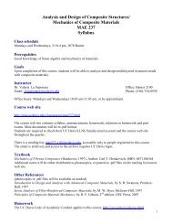
Fig. 5.8 shows the geometric interpretation of the criterion: safe loads correspond to combinations inside an
ellipse in the non-dimensional load space, non-dimensional axial force N1/(πR 2 σallow) versus non-dimensional
torque M1/(πR 3 σallow).
Shaft under torsion and bending
Consider a circular shaft subjected to both bending and torsion, as would occur, for instance, in a cantilever
shaft with a tip pulley. Let M3 and M1 be the applied bending moment and torque, respectively. The
corresponding stresses are
σ = 2M3
, and
πR3 respectively. Von Mises criterion then requires
2M1
τ = ,
πR3 (5.47)
( 2M3
πR2 )2 + 3( 2M1
1/2 )2 ≤ σallow
πR3 (5.48)

5.3. TORSION OF BARS WITH ARBITRARY CROSS-SECTIONS 133
NONDIMENSIONAL TORQUE
0.25
0.2
0.15
0.1
0.05
0
−0.05
−0.1
−0.15
−0.2
−0.25
−1 −0.8 −0.6 −0.4 −0.2 0 0.2 0.4 0.6 0.8 1
NONDIMENSIONAL AXIAL FORCE
Figure 5.8: Failure criterion in the non-dimensional load space. Loading combinations inside the ellipse
correspond to safe conditions.
for safe service load conditions. Here again, these safe load conditions corresponds to the inner portion of
an ellipse
M3
4
πR3 2
M1
+ 12
σallow πR3 2 ≤ 1,
σallow
(5.49)
in the non-dimensional loading space, non-dimensional bending moment M3/(πR 3 σallow) versus non-dimensional
torque M1/(πR 3 σallow).
5.2.2 Problems
Problem 5.1
Q Q
2R pi Figure 5.9: Pressure vessel subjected to an external torque.
Consider the pressure vessel subjected to an internal pressure pi and an external torque Q, as depicted in fig. 5.9.
The pressure vessel is of radius R and wall thickness t. Use Von Mises criterion to compute the failure envelope in
the space defined by Q/(tR 2 σallow) and piR/(tσallow).
5.3 Torsion of bars with arbitrary cross-sections
When analyzing the torsional behavior of circular cylinders, the circular symmetry of the problem led to the
conclusion that each cross-section rotates about its own center like a rigid disk. If this type of deformation
t

134 CHAPTER 5. TORSION
were assumed to remain valid for a bar of arbitrary cross-section, the displacement field, eqs. (5.4) and (5.3),
and the corresponding strain field, eqs. (5.5) to (5.7), would also describe the kinematics of bars with arbitrary
sections. The only non-vanishing stress component would be the circumferential shearing stress given by
eq. (5.12).
Unfortunately, this assumption can lead to grossly erroneous results because it implies a solution that
violates the equilibrium equations of the problem at the edge of the section. Consider, for instance, the torsion
of a rectangular bar as depicted in fig. 5.10. The circumferential shearing stress, τα, given by eq. (5.12) is
shown at an edge of the section, and it is resolved into its Cartesian components, τ12 and τ13. The shear
stress component, τ13, normal to the edge of the section and its complementary component shown acting on
the outer surface of the bar must clearly vanish since the outer surfaces of the bar are stress free. Hence,
the only allowable shearing stress component along the edge is τ12, and the stress distribution in eq. (5.12)
therefore violates equilibrium conditions along the edges of the section.
i 3
i 1
i 2
Figure 5.10: Shearing stresses along the edge of a rectangular section.
5.3.1 Saint-Venant’s solution
The solution to the problem of torsion of a bar with a cross-section of arbitrary shape was first given by
Saint-Venant.
Kinematic description
Consider a solid bar with a cross-section of arbitrary shape denoted A. A closer look at the problem and
experimental tests reveal that for a bar with an arbitrary section, each cross-section rotates like a rigid body,
but the cross-section is allowed to warp out of its own plane. This type of deformation is described by the
following assumed displacement field
13
r
12
13
u1(x1, x2, x3) = Ψ(x2, x3) κ1(x1); (5.50)
u2(x1, x2, x3) = −x3φ1(x1); u3(x1, x2, x3) = x2φ1(x1). (5.51)
The in-plane displacement field, eq. (5.51), describes a rigid body rotation of the cross-section, as was the
case for the circular cylinder (see eq. (5.3)). However, the out-of-plane displacement field does not vanish.
Instead, it is assumed to be proportional to the twist rate, κ, and has an arbitrary variation over the crosssection
described by the unknown warping function Ψ(x2, x3). This warping function will be determined by

5.3. TORSION OF BARS WITH ARBITRARY CROSS-SECTIONS 135
enforcing equilibrium conditions for the resulting shearing stress field. It will be further assumed that the
twist rate is constant along the axis of the bar, i.e. κ1(x1) = κ1. This restriction results in what is known
as the uniform torsion problem.
The strain field associated with the assumed displacement field can be calculated by applying the straindisplacement
equations (eqs. (1.51) and (1.58)) to the assumed displacement field, eqs. (5.50) and (5.51) to
yield
ε1 = 0; (5.52)
∂Ψ
γ12 =
∂x2
ε2 = 0; ε3 = 0; γ23 = 0; (5.53)
− x3
∂Ψ
κ1; γ13 = + x2 κ1. (5.54)
∂x3
The vanishing of the axial strain, eq. (5.52), is a direct consequence of the uniform torsion assumption,
whereas the vanishing of the in-plane strains, eq. (5.53) stems from the rigid body rotation assumption for
the in-plane motion of the section. The only non-vanishing strain components, γ12 and γ13, depend on the
partial derivatives of the unknown warping function.
The stress field
For bars made of a linear elastic, isotropic material, Hooke’s law, eq. (1.91), is assumed to apply. The stress
field is then found from the strain field as
σ1 = 0; (5.55)
τ12 = Gκ1
σ2 = 0; σ3 = 0; τ23 = 0; (5.56)
∂Ψ
∂x2
− x3
∂Ψ
; τ13 = Gκ1 + x2 . (5.57)
∂x3
This stress field must satisfy general equilibrium equations, eqs. (1.7), at all points of the section. Neglecting
body forces, and in view of eq. (5.55), two of the three equilibrium equations are satisfied and the remaining
one reduces to
∂τ12
+
∂x2
∂τ13
= 0. (5.58)
∂x3
Hence, using eqs. (5.57) in (5.58), the warping function must satisfy the following partial differential equation
∂ 2 Ψ
∂x 2 2
+ ∂2 Ψ
∂x 2 3
= 0. (5.59)
at all points of the cross-section.
The relevant boundary conditions can be developed by requiring that equilibrium conditions must also
be satisfied along the outer edge of the section that defines the contour C. Fig. 5.11 shows a portion of the
outer contour, C, and a curvilinear variable, s, that measures length along this contour. As illustrated in
fig. 5.10, the normal component of shear stress must vanish at all points on C, i.e.
τn = 0, (5.60)
whereas the component of shearing stress, τs, tangent to the contour does not necessarily vanish. In terms
of Cartesian components, the normal component of shearing stress, see fig. 5.11, is
dx3
τn = τ12 sin β + τ13 cos β = τ12 + τ13 −
ds
dx2
= 0. (5.61)
ds
Introducing eq. (5.57) then yields the following boundary condition for the warping function
∂Ψ
∂x2
− x3
dx3
ds −
∂Ψ dx2
+ x2 = 0. (5.62)
∂x3 ds

136 CHAPTER 5. TORSION
The warping function, Ψ(x2, x3), which yields a stress field satisfying all equilibrium requirements is the
solution of the following partial differential equation and associated boundary condition
∂Ψ
∂x2
− x3
∂2Ψ ∂x2 +
2
∂2Ψ ∂x2 = 0; on A
3
dx3
ds −
. (5.63)
∂Ψ dx2
+ x2 = 0. along C
∂x3 ds
The solution of this problem is rather complicated in view of the complex boundary condition that must
hold along C.
i 3
s
n
dx 3 ds
-dx 2
Figure 5.11: Equilibrium condition along the outer contour C.
An alternative formulation of the problem that leads to simpler boundary conditions is found by introducing
a stress function, Φ, proposed by Prandtl. This function, Φ(x2, x3), is defined as
C
s
13
i 2
n
τ12 = ∂Φ
; τ13 = −
∂x3
∂Φ
. (5.64)
∂x2
This choice may not make sense at first, but when eqs. (5.64) are substituted into the local equilibrium
equation, eq. (5.58), it is quickly apparent that the equilibrium equation is satisfied identically. Thus, shear
stresses derived from this stress function automatically satisfy the equilibrium equation, eq. (5.58). Now, if
the expressions (5.57) for the shear stresses τ12 and τ13 in terms of the warping function, Ψ, are equated to
(5.64) for the shear stresses expressed in terms of the stress function, the result is two equations
Gκ1
∂Ψ
∂x2
− x3
12
= ∂Φ
∂Ψ
; Gκ1 + x2 = −
∂x3 ∂x3
∂Φ
. (5.65)
∂x2
The warping function, Ψ, can be eliminated by taking the partial derivative of the first with respect to x3
and taking the partial derivative of the second with respect to x2. The resulting mixed partial derivative
of Ψ can then be eliminated from both equations to yield a single partial differential equation for the stress
function
∂ 2 Φ
∂x 2 2
+ ∂2 Φ
∂x 2 3
The boundary conditions along C then follow from eqs. (5.61) and (5.64)
0 = τn = ∂Φ
∂x3
dx3
ds
= −2Gκ1. (5.66)
∂Φ dx2
+
∂x2 ds
dΦ
= . (5.67)
ds
which implies a constant value of Φ along the contour C. If the section is bound by several disconnected
curves, the stress function must be a constant along each individual curve, although the value of the constant

5.3. TORSION OF BARS WITH ARBITRARY CROSS-SECTIONS 137
can be different for each curve. For solid cross-sections bound by a single curve, the constant value of the
stress function along that curve may be chosen as zero because this choice has no effect on the resulting stress
distribution. The stress function is the solution of the following partial differential equation and associated
boundary condition
Sectional equilibrium
∂ 2 Φ
∂x 2 2
+ ∂2Φ = −2Gκ1. on A
∂x 2 3
dΦ
ds
= 0 along C.
(5.68)
The differential equations for the warping and stress functions were found from local equilibrium consideration.
Global equilibrium of the section must also be verified. For a solid section bound by a single contour,
the resultant shearing forces acting on the section are
and
V2 =
V3 =
τ12 dA =
A
τ13 dA =
A
x2
x2
x3
x3
∂Φ
∂x3
− ∂Φ
∂x2
dx2dx3 =
x2
dx2dx3 = −
x3
x3
∂Φ
∂x3
x2
∂Φ
∂x2
dx3
dx2
dx2 = 0, (5.69)
dx3 = 0; (5.70)
where the last equalities follow from selecting a zero value for the stress function along the contour C. The
total torque acting on the section is
∂Φ ∂Φ
M1 =
−x2 − x3 dA. (5.71)
∂x2 ∂x3
Integrating by parts then yields
M1 = 2
(x2τ13 − x3τ12) dA =
A
A
Φ dA −
x3
A
[x2Φ] x2 dx3
−
x2
[x3Φ] x3 dx2. (5.72)
For solid cross-sections bound by a single curve, the constant value of the stress function along that curve
may be chosen as zero, and the boundary terms disappear, leading to the simple result
M1 = 2 Φ dA, (5.73)
A
i.e. the applied torque equals twice the “volume” under the stress function, Φ(x2, x3). It should be noted
that this formula only applies to solid cross-sections bound by a single curve. Indeed, if the section is bound
by several connected curves, the stress function equals a different constant along each individual curve, and
the boundary terms no longer vanish. For such sections, the applied torque should be evaluated with the
help of eq. (5.71) rather than (5.73).
In summary, the stress distribution in a bar of arbitrary cross-section subjected to uniform torsion can
be obtained by evaluating either the warping or stress functions from eqs. (5.63) or (5.68), respectively. The
stress field then follows from eqs. (5.57) or (5.64), respectively. Since all governing equations are satisfied,
this represents an exact solution of the problem as formulated from the assumed displacement field.
5.3.2 Examples
Example 5.1: Torsion of an elliptical bar
Consider a bar with an elliptical cross-section as shown in fig. 5.12. The equation for the contour C defining
the section is
x2
2
+
a
x3
2
= 1.
b

138 CHAPTER 5. TORSION
A stress function of the following form is assumed
x2 Φ = A
a
b
B
i 3
a
A
Figure 5.12: A bar with an elliptical cross-section.
2
+
x3
2
− 1 ,
b
where A is an unknown constant. The boundary condition, eq. (5.67), is clearly satisfied since Φ = 0 along
C. Substituting this in the governing differential equation, eq. (5.68), it follows that this is satisfied for the
following value of the constant, A
A
The stress function then becomes
2 2
+
a2 b2
Φ = − a2 b 2
a 2 + b 2
= −2Gκ1; =⇒ A = − a2 b 2
x2
The torque can now be computed from eq. (5.73) as
M1 = − 2a2b2 a2 x2 Gκ1
+ b2 a
Note that
A
dA = πab;
A
a
A
2
+
x3
2
− 1
b
2
x 2 2 dA = πa3 b
4 ;
+
i 2
a2 Gκ1.
+ b2
x3
2
− 1
b
A
Gκ1. (5.74)
dA.
x 2 3 dA = πab3
4 ;
are the area, and the second moments of area about ī2 and ī3, respectively, for the ellipse. Using these, the
torque then can be written as
M1 = G πa3 b 3
a 2 + b 2 κ1 = J κ1,
where the torsional stiffness of the elliptical section is now defined as
J = G πa3b3 a2 . (5.75)
+ b2 Using these results, the stress function can be expressed in terms of the applied torque
Φ = − 1
x2 2
x3
2
+ − 1 M1.
πab a b
The stress distribution is found from eqs. (5.64)
τ12 = − 2x3
πab 3 M1; τ13 = 2x2
πa 3 b M1,

5.3. TORSION OF BARS WITH ARBITRARY CROSS-SECTIONS 139
and the maximum shear stress occurs at the extreme values of x2 and x3 which occur at the boundary of
the section. The shear stress distribution is shown in fig. (5.13). Thus, at points A and B the stresses are
τ B 12 = − 2M1
πab 2 ; τ A 13 = 2M1
πa 2 b .
Somewhat surprisingly, the maximum shear stress occurs at the end of the minor axis of the ellipse, i.e. at
point B where
|τmax| = 2M1
.
πab2 This is in contrast to the torsion of a bar with circular cross-section where the maximum shear stress occurs
at points with the largest radius. Fig. (5.13b) shows a contour plot of the stress along with superposed
arrows showing the direction of the maximum shear stress. For this section, as for the circular section, the
directions are parallel to the section outline when considered along any radial line.
12
B
13
(a) Shear stress magnitude
i 3
A
i 2
i 3 axis
i2 axis
(b) Shear contours
Figure 5.13: Shear stress and warping distributions on elliptic cross section.
Finally, the warping function can be obtained by integrating eq. (5.65). Substituting the calculated stress
function (5.74) into these equations yields
∂Ψ
∂x2
= − a2 − b2 a2 x3;
+ b2 ∂Ψ
∂x3
= − a2 − b2 a2 x2.
+ b2 The first equation can be integrated with respect to x2 and the second with respect to x3 to yield
and the second with respect to x2 to yield
Ψ = − a2 − b 2
a 2 + b 2 x2x3 + f(x3)
Ψ = − a2 − b 2
a 2 + b 2 x2x3 + g(x2).
These two solutions for Ψ must be equal,and this is only possible if f(x2) = g(x3) = 0 which yields the result
Ψ = − a2 − b2 a2 x2x3.
+ b2 The warping displacement, u1(x2, x3), can now be written by substituting this result for Ψ into eq. (5.50)
a
u1(x2, x3) = −κ1
2 − b2 a2 + b2 x2x3. (5.76)
This result shows that the warping is zero on the ī2 and ī3 axes, and that it is negative in the first quadrant
(where both x2 and x3 are positive). It then alternates sign in the second, third and fourth quadrants.

140 CHAPTER 5. TORSION
warping
0.5
0
-0.5
-1
i3 axis
0.5
0
-0.5
-1.5
-1
-0.5
0
0.5
i axis
2
1
1.5
2
i 3 axis
i 2 axis
Figure 5.14: Warping distribution on elliptic cross section.
Fig. 5.14 shows a surface plot of the warping on the left (with a contour plot immediately below it) and a
separate contour plot on the right.
For a = b = R the bar with an elliptical section becomes a circular cylinder of radius R. The torsional
stiffness for the elliptical section reduces to eq. (5.21), and the maximum shear stress to eq. (5.27). Finally,
the warping function vanishes, and this is fully consistent with the symmetry arguments made for the circular
cylinder that the warping must be zero.
Example 5.2: Torsion of a thick cylinder
C o
C i
t
R i
i 3
R m
R 0
Figure 5.15: Cross-section of a circular tube.
Consider a circular tube of inner radius Ri and outer radius Ro made of a homogeneous, isotropic material
of shearing modulus G, as shown in fig. 5.15. Note that this section is bounded by two curves, Ci and Co, as
shown on the figure, that denote the inner and outer circles bounding the section. The stress function for
this problem is assumed to be in the following form: Φ = Ar 2 , where r 2 = x 2 2 + x 2 3 and A is an unknown
constant. The values of the stress function along curves Ci and Co are Φi = Ar 2 i and Φo = Ar 2 o, respectively.
Since A, ri and ro are constants, this implies that the boundary conditions on the stress function, given by
eq. (5.68), are satisfied: dΦi/dsi = dΦo/dso = 0, where si and so are curvilinear variables along Ci and Co,
respectively. Note that the boundary condition requires Φ to be constant along curves Ci and Co, but this
does not imply that Φi = 0 or Φo = 0 or Φi = Φo.
Introducing the assumed stress funtion into the governing partial differential equation (5.68) yields
2A + 2A = −2Gκ1.
Hence, the stress function becomes Φ = −Gκ1r 2 /2. This represents the exact solution of the problem, since
the stress function satisfies the governing partial differential equation and boundary conditions. The shear
stress distribution then follows from eq. (5.64) as τ12 = −Gκ1x3 and τ13 = Gκ1x2. The torque generated by
i 2

5.3. TORSION OF BARS WITH ARBITRARY CROSS-SECTIONS 141
this shear stress distribution is evaluated with the help of eq. (5.71) to find
M1 =
2π Ro
0
Ri
(x2τ13 − x3τ12) rdrdθ =
2π Ro
0
Ri
Gκ1(x 2 2 + x 2 3) rdrdθ = π
2 Gκ1(R 4 o − R 4 i ).
It should be noted here that using eq. (5.73) to evaluate the torque will yield incorrect results, as can be
easily verified. This is due to the fact that eq. (5.73) was derived assuming a solid cross-section bound by a
single curve; this is not the case for the present thick tube that is bound by two curves, Ci and Co.
The torsional stiffness of the thick tube is J = πG(R4 o − R4 i )/2, and the shear stress distribution can now
be expressed in terms of the applied torque as
2M1
τ12 = −
π(R4 o − R4 i ) x3;
2M1
τ13 =
π(R4 o − R4 x2.
i )
As expected, these results obtained using the stress function approach exactly match those obtained in
section 5.1 for the torsion of circular cylinders.
5.3.3 Saint-Venant’s solution: an energy approach
In section 5.3.1, the problem of uniform torsion of a bar of arbitrary cross-section was derived in terms of an
assumed warping (displacement) function, Ψ, and a stress function Φ(x2, x3). This stress function satisfies
the equilibrium equations by its definition, but it must also satisfy the partial differential equation, eq. (5.66),
with boundary conditions, eq. (5.67). The partial differential equation is rather difficult to solve except for
very simple sectional geometries (such as the elliptical shape treated in the previous example). It is possible,
however, to obtain approximate solutions to this difficult problem using an energy approach. In this case,
the unknown is the warping function, Ψ, and so the theorem of minimum total potential will be employed.
Based on the kinematic assumptions, eqs. 5.50 and 5.51, discussed in section 5.3.1, the only non-vanishing
strain components are the shearing strains, γ12 and γ13 (see eq. (5.54)). It follows that the strain energy
contained in a “slice” of the cross-section of length, dx1, under torsion can be written as
A = 1
2
(τ12γ12 + τ13γ13) dA. (5.77)
A
Next, just as before, the section is assumed to be made of homogeneous isotropic linear elastic material, and
hence the expression for the strain energy becomes
A = 1
1
2 G (τ 2 12 + τ 2 13) dA. (5.78)
A
Expressing the shear stresses in terms of the stress function with the help of eq. (5.64) yields
A = 1
2
1
(
G
∂Φ
)
∂x2
2 + ( ∂Φ
)
∂x3
2
dA. (5.79)
A
Next, the work done by the externally applied torque on the same “slice” can be expressed as
dφ1
W = M1 = M1κ1. (5.80)
dx1
For solid cross-sections bound by a single curve, the torque, M1, can be expressed in terms of the stress
function by eq. (5.73) to yield
W = 2κ1 Φ dA. (5.81)
The total potential energy of the system (the slice) can now be written as, Π = A − W , where −W is the
potential of external forces or the negative of the work done by them (see eq. (3.123). As a result
Π = 1
1
(
2 G
∂Φ
)
∂x2
2 + ( ∂Φ
)
∂x3
2
dA − 2κ1 Φ dA. (5.82)
A
A
A

142 CHAPTER 5. TORSION
According to the principle of minimum total potential energy, the deformation that corresponds to the
equilibrium configuration of the system will make the total potential energy a minimum. In this case, the
deformation is the assumed warping, Ψ, but since this is directly related to the stress function, Φ, we can
choose approximations for either. Following the general procedure described in section 3.6.10, approximate
solutions to the torsional problem can be obtained by starting from an assumed structure of the stress
function, then minimizing the total potential energy. This procedure will be demonstrated in the examples
below.
The expression of the total potential energy given by eq. (5.82) is valid for solid cross-sections bounded
by a single curve. For such sections, the assumed stress function should be chosen with Φ = 0 along C.
For sections bound by several disconnected curves, the applied torque should be evaluated with the help of
eq. (5.71), and the stress function equals a different constant along each individual curve.
5.3.4 Examples
Example 5.3: Torsion of rectangular section - a crude solution
Consider a bar with a rectangular cross-section of length 2a and width 2b as depicted in fig. 5.16. The
following expression will be assumed for the stress function
Φ(η, ζ) = c0(η 2 − 1)(ζ 2 − 1),
where c0 is an unknown constant, η = x2/a is the nondimensional coordinate along the ī2 axis, and ζ = x3/b is
that along the ī3 axis. This choice of the stress function implies that Φ(η = ±1, ζ) = 0 and Φ(η, ζ = ±1) = 0,
i.e. it vanishes along C.
2b
B
2a
Figure 5.16: Bar with a rectangular cross-section.
Since this is a solid cross-section bounded by a single curve, the total potential energy is given by eq. (5.82)
and is evaluated as
Π =
c2 2
0 4η
2G a2 (ζ2 − 1) 2 + 4ζ2
b2 (η2 − 1) 2
dA − 2c0κ1 (η 2 − 1)(ζ 2 − 1) dA.
A
After integration over the cross-section, this becomes
Π = c2 0
2G
8 16b
3a 15
+ 16a
15
i 3
C
A
A
i 2
8 4a 4b
− 2c0κ1
3b 3 3 .
In order to minimize the total potential energy with respect to the choice of the constant c0, the following
condition must be met: ∂Π/∂c0 = 0. This lead to a linear equation for c0
2c0 8 16b 16a 8 16ab
+ − 2κ1 = 0.
2G 3a 15 15 3b 9
Solving for c0, the stress function becomes
a 2 b 2
Φ(η, ζ) = 5
4 a2 + b2 Gκ1 (η 2 − 1)(ζ 2 − 1).

5.3. TORSION OF BARS WITH ARBITRARY CROSS-SECTIONS 143
For this section bound by a single curve, the externally applied torque is given by eq. (5.73)
M1 = 2 Φ dA =
A
5 a
2
2b2 a2
Gκ1 (η
+ b2 A
2 − 1)(ζ 2 − 1) dA = 40 a
9
3b3 a2 Gκ1.
+ b2 Since the sectional torsional stiffness J is defined as the constant of proportionality between the torque and
the twist rate, it follows that
J = 40 a
9
3b3 a2 G. (5.83)
+ b2 The stress field is now readily found from the derivatives of the stress function
τ12 = 1 ∂Φ 9
=
b ∂ζ 16
M1
ab 2 (η2 − 1)ζ; τ13 = − 1
a
∂Φ
∂η
9 M1
= −
16 a2b η(ζ2 − 1),
where the twist rate was expressed in terms of the applied torque as κ1 = M1/J.
Example 5.4: Torsion of rectangular section, a refined solution
Consider once again a bar with a rectangular cross-section of length 2a and width 2b as depicted in fig. 5.16.
The following expression will be assumed for the stress function
Φ(η, ζ) = (ζ 2 − 1)g(η),
where g(η) is an unknown function, η = x2/a the non-dimensional coordinate along the ī2 axis, and ζ = x3/b
that along the ī3 axis. This choice of the stress function implies that Φ(η, ζ = ±1) = 0 and since Φ(η = ±1, ζ)
must vanish, it follows that g(η = ±1) = 0.
Since this is a solid cross-sections bound by a single curve, the total potential energy given by eq. (5.82)
and is evaluated as
Π =
A
(ζ 2 − 1)
2 g′2
4ζ2
+
a2 b
2 g2
dA − 2κ1
A
(ζ 2 − 1)g(η) dA,
where the notation (.) ′ denotes a derivative with respect to η. The integration over the variable ζ can be
performed to yield the total potential energy as
Π = ab
+1
16
2G 15a2 g′2 + 8
+1
g2 dη − 2κ1ab (−
3b2 4
)g dη.
3
−1
In order to minimize the total potential energy with respect to the choice of the unknown function g(η), it is
necessary to resort to the Calculus of Variations. The minimum of Π(g(η)) can be determined by requiring
that the first variation vanish: δΠ = 0. This implies
δΠ = ab
2G
+1
−1
16
15a 2 2g′ δg ′ + 8
3b
Integration by parts of the first term then leads to
+1
−1
− 16
15a2 g′′ + 8
3b
−1
4
2gδg + 4Gκ1
2 3 δg
dη = 0.
8
16
g + Gκ1 δg dη +
2 3
15a2 g′ +1
δg = 0.
−1
The variation, δg, is entirely arbitrary, and hence the integrand must vanish. This yields a differential
equation (the Euler Equation) that the unknown function, g(η), must satisfy
g ′′ − γ 2 g = γ 2 b 2 Gκ1,
where γ = 5/2 a/b. The second term in the variation must also be zero. This term yields the required
boundary conditions for g(η) at η = +1 and η = −1. In this case the requirement is that either g must be
specified (δg = 0) or the derivative, g ′ , must vanish.

144 CHAPTER 5. TORSION
The general solution of the differential equation is g(η) = C1 sinh γη+C2 cosh γη−b2Gκ1, where C1 and C2
are the integration constants that can be evaluated with the help of the boundary conditions, g(η = ±1) = 0.
If follows that g(η) = (cosh γη/ cosh γ − 1) b2Gκ1, and the stress function becomes
cosh γη
Φ(η, ζ) = − 1 (ζ
cosh γ 2 − 1) b 2 Gκ1.
This stress function is shown in fig. 5.17.
Φ
0.25
0.2
0.15
0.1
0.05
0
1
0.5
0
x 3
−0.5
−1
−2
−1
x 2
0
1
2
x 3
1
0.8
0.6
0.4
0.2
0
−0.2
−0.4
−0.6
−0.8
−1
−2 −1.5 −1 −0.5 0
x
2
0.5 1 1.5 2
Figure 5.17: Left figure: stress function Φ. Right figure: distribution of shear stress over cross-section. The
arrows represent the shear stresses; the contours represent constant values of the stress function Φ. a = 2,
b = 1.
For this section bound by a single curve, the externally applied torque is given by eq. (5.73)
M1 = 2 Φ dA = 16ab3
tanh γ
1 − Gκ1.
3 γ
A
Since the sectional torsional stiffness J is defined as the constant of proportionality between the torque and
the twist rate, it follows that
J = 16ab3
tanh γ
1 − G.
3 γ
(5.84)
The stress field is now readily found from the derivatives of the stress function
τ12 = 3 M1
8 ab2 cosh γη/ cosh γ − 1
1 − (tanh γ)/γ
ζ; τ13 = − 3 M1
16 a2b γ sinh γη/ cosh γ
1 − (tanh γ)/γ (ζ2 − 1),
where the twist rate is expressed in terms of the applied torque as κ1 = M1/J. The shear stress distribution
is displayed in fig. 5.17.
Comparison of approximate solutions
The solution of the last two examples are now compared. Instead of using a and b which are the half-lengths
of the cross-section, the full length of the section a ′ = 2a and the width b ′ = 2b will be used instead. The
nondimensional torsional stiffnesses are
J1
a ′ b ′3 =
G 5
18
1
1 + (b ′ /a ′ ;
) 2
J2
a ′ b ′3 =
G 1
1 −
3
tanh γ
. (5.85)
γ
J1 is the torsional stiffness obtained with the crude solution, see eq. (5.83), whereas J2 is that obtained
with the refined solution, see eq. (5.84). For a very thin strip, b → 0 and a/b → ∞. It follows that

5.3. TORSION OF BARS WITH ARBITRARY CROSS-SECTIONS 145
J1/a ′ b ′3 G → 5/18 and J2/a ′ b ′3 G → 1/3. Fig. 5.18 shows the torsional stiffnesses predicted by the crude and
refined solutions as a function of a ′ /b ′ = a/b. The exact solution of the problem is also shown for reference.
While all solutions are in good agreement for aspect ratios near unity, the crude solution significantly under
predicts the stiffness for higher aspect ratios. Note the excellent accuracy of the refined solution compared
to the exact solution.
NONDIMENSIONAL STIFFNESS
0.3
0.25
0.2
0.15
0.1
0.05
0
1 2 3 4 5 6 7 8 9 10 11 12
a/b
Figure 5.18: Nondimensional torsional stiffness versus aspect ratio a/b for the crude (◦), refined (△) and
exact (▽) solutions.
The maximum values of the shear stress components τ12 and τ13 are found at points B and A, respectively,
see fig. 5.16. The predictions at point B are
a ′ b ′2 |τB1|
M1
= 9
2 ;
a ′ b ′2 |τB2|
M1
= 3
1 − 1/ cosh γ
, (5.86)
1 − (tanh γ)/γ
where τB1 and τB2 are the stress components predicted by the crude and refined solutions, respectively.
Fig. 5.19 shows the predictions of the crude and refined solutions, together with the exact solution. Here
again, good agreement is found between the refined and exact solutions, except when a ≈ b. In fact, for
a = b, the refined solution underestimates the stress by about 10%.
NONDIMENSIONAL SHEAR STRESS AT B
5
4.8
4.6
4.4
4.2
4
3.8
3.6
3.4
3.2
3
1 2 3 4 5 6 7 8 9 10 11 12
a/b
Figure 5.19: Non-dimensional shear stress at point B versus aspect ratio a/b for the crude (◦), refined (△)
and exact (▽) solutions.

146 CHAPTER 5. TORSION
The predictions at point A are
a ′ b ′2 |τA1|
M1
= 9 b
2
′ 9 b
=
a ′ 2 a ;
a ′ b ′2 |τA2|
M1
= 3
5
2 2
tanh γ
, (5.87)
1 − (tanh γ)/γ
where τA1 and τA2 are the stress components predicted by the crude and refined solutions, respectively.
Fig. 5.20 shows the predictions of the crude and refined solutions, together with the exact solution. Here
again, good agreement is found between the refined and exact solutions. Comparing the results at points
A and B, it is clear that the maximum shear stress component occurs in the middle of the long side of the
rectangular section, i.e. at point B if a > b.
NONDIMENSIONAL SHEAR STRESS AT A
5.5
5
4.5
4
3.5
3
2.5
2
1.5
1
0.5
0
1 2 3 4 5 6 7 8 9 10 11 12
a/b
Figure 5.20: Nondimensional shear stress at point A versus aspect ratio a/b for the crude (◦), refined (△)
and exact (▽) solutions.
5.3.5 Problems
Problem 5.2
b
i 3
B
b
r
Figure 5.21: Circular shaft with a keyway.
Consider a circular shaft of radius a with a semi-circular keyway of radius b, as depicted in fig. 5.21. The shaft
is subjected to torsion.
(1) Find the stress function for this problem starting from
a
a
Φ = A x 2 2 + x 2 3 − 2ax2 1 − b2
x 2 2 + x2 3
A
r
i 2
.

5.4. TORSION OF A THIN RECTANGULAR CROSS-SECTION 147
(2) Find the shear stress distribution τr = τr(α) and τα = τα(α) along the contour Γa of the shaft. (3) Find the
shear stress distribution τr = τr(β) and τβ = τβ(β) along the contour Γb of the keyway. (4) Let τN = Gκ1a be the
shaft maximum shearing stress in the absence of keyway. Find
Comment on your results.
Problem 5.3
τ
lim
b→0
A α τ
; lim
τN b→0
B β
.
τN
The narrow rectangular strip (a ≫ b) shown in fig. 5.16 is the cross-section of a bar subjected to torsion. Investigate
the behavior of this section under torsion using an energy approach. Use a stress function of the following type
Φ = Gκ1 b 2 − x 2 3 1 − e −α(a−|x2|)
where α is an unknown parameter. Assume e −αa ≈ 0.
(1) Find the torsional stiffness of the bar. (2) Find the shearing stresses at points A and B, [(2a)(2b) 2 τA]/M1
and ([(2a)(2b) 2 τB]/M1, respectively, where M1 is the applied torque.
Problem 5.4
Am exact solution for the torsion of a bar with a rectangular cross-section depicted in fig. 5.16 can be found by
considering the following series expansion for the stress function
Φ(η, ζ) =
∞
gn(η) cos αnζ,
n=1
where gn(η) are unknown functions, αn = (2n − 1)π/2, η = x2/a the nondimensional coordinate along the ī2 axis,
and ζ = x3/b that along the ī3 axis. Use the energy approach to show that
Φ(η, ζ) = 4b 2 Gκ1
The nondimensional torsional stiffness then follows
¯J =
J
Ga ′ = 2
b ′3
∞
n=1
∞ (−1) n+1
n=1
1
α 4 n
−
α 3 n
tanh βn
α 4 nβn
1 −
cosh βnη
cosh βn
= 1
3
− 2
,
∞
n=1
cos αnζ.
tanh βn
α4 ,
nβn
where a ′ = 2a and b ′ = 2b are the length and width of the section, respectively. This solution is plotted in fig. 5.18.
The shear stress at point A is found to be
a ′ b ′2 |τA|
M1
= 2
¯J
∞
n=1
1
α 2 n
whereas the shear stress component at point B is
a ′ b ′2 |τB|
M1
= 2
¯J
∞
n=1
(−1) n+1
α 2 n
−
1
α 2 n cosh βn
− (−1) n+1 1 − tanh βn
α 2 n
= 1 2
¯J
−
¯J
= 0.742454
¯J
∞
1
α
n=1
2 n cosh βn
− 2
¯J
,
∞
(−1) n+1 1 − tanh βn
.
These stress components are shown in figs. 5.20 and 5.19, respectively. Note the very fast convergence of all the series
involved in this solution due to the powers of αn appearing in the denominators.
5.4 Torsion of a thin rectangular cross-section
A thin rectangular cross-section is an important case to consider because it is commonly encountered when
dealing with beams and bars constructed with thin-walled cross-sections. It turns out that a solution that is
exact in the limit as the thickness of such a cross-section becomes vanishingly small can be developed with
relatively little work.
n=1
α 2 n

148 CHAPTER 5. TORSION
b
i 3
b >>t
i 2
max
(a) (b)
Figure 5.22: (a) Thin rectangular cross section geometry. (b) Shear stress distribution through the thickness
of a thin rectangular strip.
Consider a thin rectangular cross-section as shown if fig. 5.22 where b is the long dimension, taken in the
ī3 direction, and t is the width, taken in the ī2 direction. If the width or thickness, t, can be considered to
be much smaller than b (t ≪ b), then is it reasonable to assume also that the solution for the shear stresses
and warping function are constant along the long (ī3) dimension of the problem. In other words, we can
assume that ∂/∂x3(.) = 0.
Under these assumptions, the governing equation, eq. (5.66) no longer has terms involving ∂/∂x3 and so
it reduces to an ordinary differential equation with respect to the x2 variable only
The solution to eq. (5.88) is then
d 2 Φ
dx 2 2
i 3
t
max
= −2Gκ1. (5.88)
Φ(x2) = −Gκ1x 2 2 + C1x2 + C2.
The boundary conditions require that Φ = 0 on the boundary or in this case, 0 = Φ(x2 = −t/2) = Φ(x2 =
+t/2), which results in
t
0 = Φ(t/2) = −Gκ1
2
4
t
+ C1
2 + C2,
t
0 = Φ(−t/2) = −Gκ1
2
4
i 2
t
− C1 + C2.
2
The solution for the constants is C1 = 0 and C2 = Gκ1t 2 /4 so that the solution for Φ is
Φ(x2) = −Gκ1
x 2 2 − t2
. (5.89)
4
The stress function defines the shear stress distribution on the section, and using eq. (5.64) leads to
τ12 = ∂Φ
= 0, τ13 = −
∂x3
∂Φ
= 2Gκ1x2. (5.90)
∂x2
This result shows that the only shear stress is the τ13 component and on the cross-section it acts in the ī3
direction. Thus the shear stress distribution looks like that shown in fig. 5.22 (b).
The M1 moment resultant on the cross-section can be computed using eq. (5.73)
t/2
M1 = 2 Φ dA = −2Gκ1 x
A
−t/2
2 2 − t2
b dx2 =
4
1
3 Gκ1bt 3 .

5.5. TORSION OF THIN-WALLED OPEN SECTIONS 149
Since the proportionality between the moment resultant, M1, and the twist rate, κ1, is defined as the torsional
stiffness, J, it follows that
J = 1
3 Gbt3
(5.91)
is the torsional stiffness for a bar constructed from a homogeneous material and with a thin rectangular
cross-section shape.
b >>t
b
Figure 5.23: Warping of the cross section of a thin rectangular strip.
The warping function, Ψ, can be determined by substituting the stress function solution, eq. (5.89), into
eq. (5.65) to yield two partial differential equations
the solutions of which are
∂Ψ
∂x2
= 1 ∂Φ
+ x3; and
Gκ1 ∂x3
t
i 3
∂Ψ
∂x3
i 2
= − 1 ∂Φ
− x2,
Gκ1 ∂x2
Ψ = x3x2 + f(x3), and Ψ = x2x3 + g(x2),
respectively; f(x3) and g(x2) are two arbitrary functions. Since the problem has a unique solution, the two
expressions for Ψ must be equal. This is only possible if f(x3) = g(x2) = 0, and hence, the warping function
is
Ψ = x2x3.
The axial displacement, u1(x2, x3), can be determined by substituting this result into eq. (5.50) to yield
u1(x2, x3) = Ψ(x2, x3)κ1 = κ1x2x3 = M1
J x2x3. (5.92)
This warping is very similar to that computed for the elliptical cross section. In both cases, the axes of
symmetry do not experience any warping, i.e. u1 = 0 along these axes, while each quadrant of the crosssection
experiences either a positive or a negative warping in an alternating sequence around the cross-section,
as illustrated in fig. 5.23.
5.5 Torsion of thin-walled open sections
The results of the previous section are readily extended to thin-walled open sections. The primary assumption
made in developing this solution was that the gradients of all the variables is very small in the direction
tangential to the thin wall. For the thin rectangular strip shown in fig. 5.22 (b), this means along axis ī3.
Of course, if the section were to be rotated 90 degrees so that the long direction of the strip were along axis

150 CHAPTER 5. TORSION
ī2, the gradients of all the variables would vanish in that direction. More generally, gradients of all variables
should vanish along the local tangent to the curve, C, that defined the geometry of the cross-section. Thus,
the developments of the previous section still apply to a generally curved, thin-walled open section, and the
torsional stiffness of such section becomes
J = G ℓt3
, (5.93)
3
where ℓ is the length of curve C and t the wall thickness. For the thin rectangular section, the shear stress
τ12 vanishes, leaving the sole shear stress component τ13, see eq. (5.90). For the present problem, the only
non-vanishing stress component is the tangential shear stress, τs, acting in the direction tangent to curve C.
Here again, the shear stress is not uniform across the thickness, but instead, varies linearly from zero at the
midline to maximum positive and negative values at the opposite edges of the wall, a distance ±t/2 from
the midline. At these points, the magnitude of the shear stress is
τ max
s = Gt κ1. (5.94)
The maximum shear stress can also be expressed in terms of the applied torque as
max
max
τ max
s
= 3M1
. (5.95)
bt2 Figure 5.24: Thin-walled open section composed of one curved segments and two straight segments.
A more general thin-walled open section could be composed of a number of straight and curved segments,
such as the situation illustrated in fig. 5.24. In this case, the torsional stiffness of the cross-section is the
sum of the torsional stiffnesses of the individual segments is composed of,
J =
i
Ji = 1
3
i
i 3
i 2
Giℓit 3 i , (5.96)
where Gi, ℓi and ti are the shear modulus, length and thickness of the i th segment, respectively. The shear
stress along the edge of each segment is still given by eq. (5.94), where κ1 is the twist rate of the cross-section.
Hence, the maximum shear stress will be found in the segment featuring the largest thickness
τ max
s
= Gtmax
where tmax is the thickness of the segment with the largest thickness.
M1
, (5.97)
J

5.5. TORSION OF THIN-WALLED OPEN SECTIONS 151
5.5.1 Examples
Example 5.5: Torsion of thin-walled section
Consider, as an example, the C-channel shown in fig. 5.25. The torsional stiffness of the section is given by
eq. (5.96) as
J = G 3
btf + ht
3
3 w + bt 3 G 3
f = htw + 2bt
3
3 f . (5.98)
The tangential shear stresses at the edges of the wall are given by eq. (5.94) as
τw = Gtwκ1 = Gtw
J M1; and τf = Gtf κ1 = Gtf
J M1. (5.99)
for the stresses in the web and flanges, respectively. The maximum shear stress will be found in the segment
featuring the maximum thickness.
5.5.2 Problems
Problem 5.5
h
t w
b
Figure 5.25: A thin-walled C-channel section
i 3
R
Figure 5.26: Semi-circular open cross-section.
i 3
t
s
t f
t f
i 2
i 2

152 CHAPTER 5. TORSION
Fig. 5.26 depicts the thin-walled, semi-circular open cross-section of a beam. The wall thickness is t, and the
material Young’s and shearing moduli are E and G, respectively.
(1) Find the torsional stiffness of the section. (2) Find the distribution of shear stress due to an applied torque
Q. (3) Indicate the location and magnitude of the maximum shear stress Rt 2 τmax/Q.
Problem 5.6
h 1
h 1
t
t
Figure 5.27: Cross-section of a thin-walled beam.
Fig. 5.27 depicts the cross-section of a thin-walled beam.
(1) Find the torsional stiffness of the section. (2) Find the magnitude and location of the maximum shearing
stress if the section is subjected to a torque Q. (3) Sketch the distribution of shear stress through the thickness of
the wall.
5.6 The membrane analogy
Saint-Venant’s solution expresses the shear stress distribution over the cross-section of a bar under torsion in
terms of the warping or stress functions which satisfy the partial differential eqs. (5.63) or (5.68), respectively.
Though this procedure completely solves the problem, the analyst has little intuition about the shape of the
warping or stress functions for a given cross-sectional shape.
Prandtl developed an analogy between the shape of the stress function and the deflected shape of a thin,
uniformly stretched membrane (i.e., a soap film) subjected to a uniform transverse pressure. Since the
solution of this latter problem is rather intuitive, it provides valuable insight about the shape of the stress
function.
Consider a thin, uniformly stretched membrane attached to a planar curve C defining a domain A, and
subjected to a uniform transverse pressure p, as depicted in fig. 5.28. Under the effect of the pressure,
the membrane deflects upwards and reaches an equilibrium shape u1(x2, x3) where the applied pressure is
equilibrated by the out-of-plane component of the uniform stretching force S.
i 3
i 2
b
Deflected
membrane
shape
t
h 2
h 2
i 1
u (x , x )
1 2 3
C
S Uniform
pressure p
Figure 5.28: The thin membrane attached to the contour C.
The deflected shape of the membrane can be evaluated by considering the differential element shown in
fig. 5.29. The force p dx2dx3 due to the applied pressure is equilibrated by the out-of-plane components of
i 2

5.6. THE MEMBRANE ANALOGY 153
the stretching forces
p dx2dx3 − S ∂u1
∂x2
−S ∂u1
∂x3
∂u1
dx2 + S
∂x3
∂u1
dx3 + S
∂x2
+ ∂2 u1
∂x 2 3
+ ∂2u1 ∂x2 2
dx3
dx2
dx2 = 0.
After simplification, this equilibrium condition which must hold at all points of A becomes
∂ 2 u1
∂x 2 2
+ ∂2 u1
∂x 2 3
= − p
S
dx3
(5.100)
on A. (5.101)
Along the planar curve C, the deflected shape of the membrane must remain constant, i.e.
du1
ds
= 0 along C. (5.102)
The deflected shape of the membrane can be found by solving the partial differential equation (5.101)
subjected to the boundary condition (5.102).
The membrane analogy now follows from comparing the governing equations and boundary conditions,
eq. (5.68) for the stress function with the corresponding eqs. (5.101) and (5.102) for the deflection of the
membrane. Clearly, the two sets of equations are identical if
Φ
2Gκ1
= u1
. (5.103)
p/S
This analogy implies that the stress function corresponding to the torsional problem of a bar of crosssectional
area A with an outer contour C is equal to the deflected shape of a membrane stretched over the
same contour, within a normalizing constant (2Gκ1)/(p/S).
i 1
du /dx
1 2
S
dx 2
p
i 2
S
2 2
du /dx + (d u /dx ) dx
1 2 1 2 2
Figure 5.29: A differential element of the membrane.
This analogy is further extended by considering contours of constant deflection of the membrane. Fig. 5.30
shows such a contour denoted ¯ C that encloses an area A. Let s be the curvilinear variable measuring length
along ¯ C, and ¯s and ¯n unit vectors respectively tangent and normal to ¯ C. It is clear that ∂u1/∂s = 0 since
¯C is a contour of constant membrane deflection, and ∂u1/∂n represents the slope of the membrane in the
direction normal to ¯ C. On the other hand, the components of shearing stress τn and τs in the direction
normal and tangent to ¯ C are
τn = ∂Φ
∂s ; τs = − ∂Φ
, (5.104)
∂n
where n measures length in the direction normal to ¯ C. Introducing (5.103) then yields
τn = 2Gκ1
p/S
∂u1
∂s = 0; τs = − 2Gκ1
p/S
∂u1
. (5.105)
∂n
This means that at any point, the shear stress is tangent to the contour of constant membrane deflection
passing through that point, and the magnitude of the shearing stress is proportional to the slope of the

154 CHAPTER 5. TORSION
C
A
Contour of constant
membrane deflection
i 3
s n
Figure 5.30: Contours of constant membrane deflection.
membrane in the direction normal to that contour. This conclusion also applies to C the outer contour of
the cross-section where the shearing stress is tangent to C as required by the local equilibrium condition,
eq. (5.60), and its magnitude is proportional to the slope of the membrane in the direction normal to the
outer contour.
Consider now the equilibrium of the portion A of the membrane enclosed by ¯ C. The force pA due to the
applied pressure is equilibrated by the normal component of the stretching force
pA +
¯C
¯C
S ∂u1
∂n
s
C
i 2
ds = 0. (5.106)
We then introduce the analogy (5.103) and simplify to find
1
¯ℓ
A
τs ds = 2Gκ1 ¯ℓ
. (5.107)
where ¯ ℓ is the length of the closed contour ¯ C. In other words, the average shearing stress along a contour of
constant membrane deflection is proportional to A/ ¯ ℓ, i.e. the ratio of the area enclosed by ¯ C to its perimeter.
Finally, the torque, given by eq. (5.73), is related to the volume V under the deflected membrane
5.6.1 Examples
M1 = 2
A
dA = 2Gκ1
p/S 2
Example 5.6: Torsion of a thin rectangular section
A
dA = 2Gκ1
p/S
2V. (5.108)
The torsional behavior of a thin rectangular section similar to that considered in section 5.4 will be investigated
with the help of the membrane analogy. Consider the thin rectangular strip shown in fig. 5.31, where
t ≪ b. The membrane stretched over this thin strip will deflect into a cylindrical shape with no appreciable
slope in the ī3 direction, except near the far edges of the section. This means that it is reasonable to assume
∂u1/∂x3 ≈ 0, and the governing equation for the membrane, eq. (5.101), becomes
∂ 2 u1
∂x 2 2
= − p
. (5.109)
S
Integrating and enforcing u1 = 0 at the edges of the contour, i.e. at x2 = ±t/2 then yields
u1 = 1 t
(
2 2 )2
1 − ( 2x2
t )2
p
. (5.110)
S

5.6. THE MEMBRANE ANALOGY 155
b
t
i 3
i 2
i 1
p
Figure 5.31: A thin rectangular strip.
t
Deflected
membrane
shape
The membrane analogy (5.103) then gives the corresponding stress function
The stress distribution now follows from eq. (5.64)
Φ = ( t
2 )2
1 − ( 2x2
t )2
i 2
Gκ1. (5.111)
τ12 ≈ 0; τ13 = 2x2Gκ1, (5.112)
and the torque associated with this stress distribution is evaluated with the help of eq. (5.73)
M1 = 2Gκ1( t
2 )2 b
+t/2
−t/2
1 − ( 2x2
t )2
dx2 = bt3
3 Gκ1. (5.113)
Here again a linear relationship is found between the applied torque and the resulting twist rate. The
torsional stiffness for the rectangular strip is now
J = G bt3
. (5.114)
3
The torsional stiffness is proportional to t 3 , i.e. a thin rectangular strip has a very low torsional stiffness.
Eliminating the twist rate between eqs. (5.112) and (5.113) yields the stress distribution in terms of the
applied torque
τ12 ≈ 0; τ13 = 3M1
(2x2 ). (5.115)
bt2 t
This corresponds to a distribution of shear stress that is linear through the thickness of the thin rectangular
strip, as depicted in fig. 5.22 (b). The shearing stress vanishes at the wall mid-line and reaches its maximum
value along the two edges of the section. Clearly,
τmax = 3M1
. (5.116)
bt2

156 CHAPTER 5. TORSION
The following observation gives interesting insight into the torsional behavior of thin rectangular strips.
The torque resulting from the stress distribution, eq. (5.115), is
b
+t/2
b
6M1
τ13 x2 dx2dx3 = dx3
bt3 +t/2
x 2
2 dx2 = M1
. (5.117)
2
0
−t/2
0
This means that the shearing stresses τ13 only account for half of the torque. The other half must be
associated with τ12. Though this stress component is very small, its contribution to the torque is multiplied
by a moment arm b/2, as compared to the moment are t/2 for the τ13 component.
Finally, the membrane analogy provides further insight into the behavior of bars with non circular cross
sections. Specifically, consider the distribution of shear stress in the regions on the cross section near a
convex corner, for example, a corner of a rectangular section. It should be intuitively obvious that the slope
of a membrane in this area will be relatively flat compared the the slope near the midpoints of the long edges,
for example. Since the direction of the shear stress is along a contour of the membrane and the magnitude
is proportional to the slope perpendicular to the contour, we can conclude that the corner regions do not
experience significant shear stresses. This situation is even more pronounced for a cross section in the shape
of an equilateral triangle. In fact, for this kind of shape, the shear stresses and torsional stiffness are not
significantly better than what would be obtained for a circular cross section sized to match the largest circle
that can be inscribed within the triangle.
−t/2