Torsion

More documents

Recommendations

Info

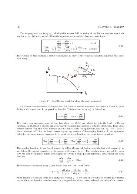
136 CHAPTER 5. TORSION The warping function, Ψ(x2, x3), which yields a stress field satisfying all equilibrium requirements is the solution of the following partial differential equation and associated boundary condition ∂Ψ ∂x2 − x3 ∂2Ψ ∂x2 + 2 ∂2Ψ ∂x2 = 0; on A 3 dx3 ds − . (5.63) ∂Ψ dx2 + x2 = 0. along C ∂x3 ds The solution of this problem is rather complicated in view of the complex boundary condition that must hold along C. i 3 s n dx 3 ds -dx 2 Figure 5.11: Equilibrium condition along the outer contour C. An alternative formulation of the problem that leads to simpler boundary conditions is found by introducing a stress function, Φ, proposed by Prandtl. This function, Φ(x2, x3), is defined as C s 13 i 2 n τ12 = ∂Φ ; τ13 = − ∂x3 ∂Φ . (5.64) ∂x2 This choice may not make sense at first, but when eqs. (5.64) are substituted into the local equilibrium equation, eq. (5.58), it is quickly apparent that the equilibrium equation is satisfied identically. Thus, shear stresses derived from this stress function automatically satisfy the equilibrium equation, eq. (5.58). Now, if the expressions (5.57) for the shear stresses τ12 and τ13 in terms of the warping function, Ψ, are equated to (5.64) for the shear stresses expressed in terms of the stress function, the result is two equations Gκ1 ∂Ψ ∂x2 − x3 12 = ∂Φ ∂Ψ ; Gκ1 + x2 = − ∂x3 ∂x3 ∂Φ . (5.65) ∂x2 The warping function, Ψ, can be eliminated by taking the partial derivative of the first with respect to x3 and taking the partial derivative of the second with respect to x2. The resulting mixed partial derivative of Ψ can then be eliminated from both equations to yield a single partial differential equation for the stress function ∂ 2 Φ ∂x 2 2 + ∂2 Φ ∂x 2 3 The boundary conditions along C then follow from eqs. (5.61) and (5.64) 0 = τn = ∂Φ ∂x3 dx3 ds = −2Gκ1. (5.66) ∂Φ dx2 + ∂x2 ds dΦ = . (5.67) ds which implies a constant value of Φ along the contour C. If the section is bound by several disconnected curves, the stress function must be a constant along each individual curve, although the value of the constant
5.3. TORSION OF BARS WITH ARBITRARY CROSS-SECTIONS 137 can be different for each curve. For solid cross-sections bound by a single curve, the constant value of the stress function along that curve may be chosen as zero because this choice has no effect on the resulting stress distribution. The stress function is the solution of the following partial differential equation and associated boundary condition Sectional equilibrium ∂ 2 Φ ∂x 2 2 + ∂2Φ = −2Gκ1. on A ∂x 2 3 dΦ ds = 0 along C. (5.68) The differential equations for the warping and stress functions were found from local equilibrium consideration. Global equilibrium of the section must also be verified. For a solid section bound by a single contour, the resultant shearing forces acting on the section are and V2 = V3 = τ12 dA = A τ13 dA = A x2 x2 x3 x3 ∂Φ ∂x3 − ∂Φ ∂x2 dx2dx3 = x2 dx2dx3 = − x3 x3 ∂Φ ∂x3 x2 ∂Φ ∂x2 dx3 dx2 dx2 = 0, (5.69) dx3 = 0; (5.70) where the last equalities follow from selecting a zero value for the stress function along the contour C. The total torque acting on the section is ∂Φ ∂Φ M1 = −x2 − x3 dA. (5.71) ∂x2 ∂x3 Integrating by parts then yields M1 = 2 (x2τ13 − x3τ12) dA = A A Φ dA − x3 A [x2Φ] x2 dx3 − x2 [x3Φ] x3 dx2. (5.72) For solid cross-sections bound by a single curve, the constant value of the stress function along that curve may be chosen as zero, and the boundary terms disappear, leading to the simple result M1 = 2 Φ dA, (5.73) A i.e. the applied torque equals twice the “volume” under the stress function, Φ(x2, x3). It should be noted that this formula only applies to solid cross-sections bound by a single curve. Indeed, if the section is bound by several connected curves, the stress function equals a different constant along each individual curve, and the boundary terms no longer vanish. For such sections, the applied torque should be evaluated with the help of eq. (5.71) rather than (5.73). In summary, the stress distribution in a bar of arbitrary cross-section subjected to uniform torsion can be obtained by evaluating either the warping or stress functions from eqs. (5.63) or (5.68), respectively. The stress field then follows from eqs. (5.57) or (5.64), respectively. Since all governing equations are satisfied, this represents an exact solution of the problem as formulated from the assumed displacement field. 5.3.2 Examples Example 5.1: <strong>Torsion</strong> of an elliptical bar Consider a bar with an elliptical cross-section as shown in fig. 5.12. The equation for the contour C defining the section is x2 2 + a x3 2 = 1. b
Page 1 and 2: Chapter 5 Torsion In the previous c
Page 3 and 4: 5.1. TORSION OF CIRCULAR CYLINDERS
Page 9 and 10: 5.2. STRENGTH UNDER COMBINING LOADI
Page 11 and 12: 5.3. TORSION OF BARS WITH ARBITRARY
Page 13: 5.3. TORSION OF BARS WITH ARBITRARY
Page 25 and 26: 5.4. TORSION OF A THIN RECTANGULAR
Page 27 and 28: 5.5. TORSION OF THIN-WALLED OPEN SE
Page 29 and 30: 5.5. TORSION OF THIN-WALLED OPEN SE
Page 31 and 32: 5.6. THE MEMBRANE ANALOGY 153 the s
Page 33 and 34: 5.6. THE MEMBRANE ANALOGY 155 b t i

Torsion

You also want an ePaper? Increase the reach of your titles

Delete template?

Save as template?