Diffraction Grating Handbook

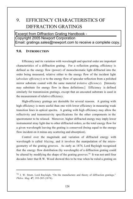
9. EFFICIENCY CHARACTERISTICS OF
DIFFRACTION GRATINGS
9.0. INTRODUCTION
Efficiency and its variation with wavelength and spectral order are important
characteristics of a diffraction grating. For a reflection grating, efficiency is
defined as the energy flow (power) of monochromatic light diffracted into the
order being measured, relative either to the energy flow of the incident light
(absolute efficiency) or to the energy flow of specular reflection from a polished
mirror substrate coated with the same material (relative efficiency). [Intensity
may substitute for energy flow in these definitions.] Efficiency is defined
similarly for transmission gratings, except that an uncoated substrate is used in
the measurement of relative efficiency.
High-efficiency gratings are desirable for several reasons. A grating with
high efficiency is more useful than one with lower efficiency in measuring weak
transition lines in optical spectra. A grating with high efficiency may allow the
reflectivity and transmissivity specifications for the other components in the
spectrometer to be relaxed. Moreover, higher diffracted energy may imply lower
instrumental stray light due to other diffracted orders, as the total energy flow for
a given wavelength leaving the grating is conserved (being equal to the energy
flow incident on it minus any scattering and absorption).
Control over the magnitude and variation of diffracted energy with
wavelength is called blazing, and it involves the manipulation of the micro-
geometry of the grating grooves. As early as 1874, Lord Rayleigh recognized
that the energy flow distribution (by wavelength) of a diffraction grating could
be altered by modifying the shape of the grating grooves. 79 It was not until four
decades later that R.W. Wood showed this to be true when he ruled a grating on
79 J. W. Strutt, Lord Rayleigh, “On the manufacture and theory of diffraction gratings,”
Philos. Mag. 47, 193-205 (1874).
124

which he had controlled the groove shape, thereby producing the first deliber-
ately blazed diffraction grating. 80
The choice of an optimal efficiency curve for a grating depends on the
specific application. For some cases the desired instrumental response is linear
with wavelength; that is, the ratio of intensity of light and the electronic signal
into which it is transformed is to be nearly constant across the spectrum. To
approach this as closely as possible, the spectral emissivity of the light source
and the spectral response of the detector should be considered, from which the
desired grating efficiency curve can be derived. Usually this requires peak
grating efficiency in the region of the spectrum where the detectors are least
sensitive; for example, a visible-light spectrometer using a silicon detector would
be much less sensitive in the blue than in the red, suggesting that the grating
itself be blazed to yield a peak efficiency in the blue.
A typical efficiency curve (a plot of absolute or relative diffracted efficiency
vs. diffracted wavelength λ) is shown in Figure 9-1. Usually such a curve shows
E
E P
λ B
Figure 9-1. A typical (simplified) efficiency curve. This curve shows the efficiency E of a
grating in a given spectral order m, measured vs. the diffracted wavelength λ. The peak
efficiency E P occurs at the blaze wavelength λ B .
80 R. Wood, “The echellette grating for the infra-red,” Philos. Mag. 20 (series 6), 770-778
(1910).
125
λ

a single maximum, at the peak wavelength (or blaze wavelength) λ B . This curve
corresponds to a given diffraction order m; the peak of the curve decreases in
magnitude and shifts toward shorter wavelengths as |m| increases. The
efficiency curve also depends on the angles of use (i.e., the angles of incidence
and diffraction). Moreover, the curve depends on the groove spacing d (more
appropriately, on the dimensionless parameter λ/d) and the material with which
the grating is coated (for reflection gratings) or made (for transmission gratings).
In many instances the diffracted power depends on the polarization of the
incident light. P-plane or TE polarized light is polarized parallel to the grating
grooves, while S-plane or TM polarized light is polarized perpendicular to the
grating grooves (see Figure 9-2). For completely unpolarized incident light, the
efficiency curve will be exactly halfway between the P and S efficiency curves.
grating
Figure 9-2. S and P polarizations. The P polarization components of the incident and
diffracted beams are polarized parallel to the grating grooves; the S components are
polarized perpendicular to the P components. Both the S and P components are perpendicular
to the propagation directions.
Usually light from a single spectral order m is used in a spectroscopic
instrument, so a grating with ideal efficiency characteristics would diffract all of
126
S
P
P
S

the power incident on it into this order (for the wavelength range considered).
In practice, this is never true: the distribution of the power by the grating
depends in a complicated way on the groove spacing and profile, the spectral or-
der, the wavelength, and the grating material.
Anomalies are locations on an efficiency curve (efficiency plotted vs.
wavelength) at which the efficiency changes abruptly. First observed by R. W.
Wood, these sharp peaks and troughs in an efficiency curve are sometimes
referred to as Wood's anomalies. Anomalies are rarely observed in P polarization
efficiency curves, but they are often seen in S polarization curves (see Figure 9-
3). Anomalies are discussed in more detail in Section 9.13.
E
3 −2 2 −1
P
S
Figure 9-3. Anomalies in the first order for a typical grating with triangular grooves.
The P efficiency curve (solid line) is smooth, but anomalies are evident in the S curve
(dashed line). The passing-off locations are identified by their spectral order at the top of
the figure.
127
λ

9.1. GRATING EFFICIENCY AND GROOVE SHAPE
The maximum efficiency of a grating is typically obtained with a simple
smooth triangular groove profile, as shown in Figure 9-4, when the groove (or
blaze) angle θ B is such that the specular reflection angle for the angle of inci-
dence is equal (in magnitude and opposite in sign) to the angle of diffraction (see
Section 2.8). Ideally, the groove facet should be flat with smooth straight edges,
and be generally free from irregularities on a scale comparable to a small fraction
(< 1/10) of the wavelength of light being diffracted.
Fraunhofer was well aware that the dis tribution of power among the various
diffraction orders depended on the shape of the individual grating grooves.
Wood, many decades later, was the first to achieve a degree of control over the
groove shape, thereby concentrating spectral energy into one angular region.
Wood's gratings were seen to light up, or blaze, when viewed at the correct
angle.
θ
FN
128
β
θ
B
GN
α
B blaze arrow
Figure 9-4. Triangular groove geometry. The angles of incidence α and diffraction β are
shown in relation to the facet angle θ Β. GN is the grating normal and FN is the facet
normal. When the facet normal bisects the angle between the incident and diffracted rays,

the grating is used in the blaze condition. The blaze arrow (shown) points from GN to
FN.
9.2. EFFICIENCY CHARACTERISTICS FOR TRIANGULAR-GROOVE
GRATINGS
Gratings with triangular grooves can be generated by mechanical ruling, or
by blazing sinusoidal groove profiles by ion etching. The efficiency behavior of
gratings with triangular groove profiles may be divided into six families, de-
pending on the blaze angle: 81
family blaze angle
very low blaze angle θ B < 5°
low blaze angle 5° < θ B < 10°
medium blaze angle 10° < θ B < 18°
special low anomaly 18° < θ B < 22°
high blaze angle 22° < θ B < 38°
very high blaze angle θ B > 38°
Very low blaze angle gratings (θ B < 5°) exhibit efficiency behavior that is
almost perfectly scalar; that is, polarization effects are virtually nonexistent.
In this region, a simple picture of blazing is applicable, in which each groove
facet can be considered a simple flat mirror. The diffracted efficiency is greatest
for that wavelength that is diffracted by the grating in the same direction as it
would be reflected by the facets. This efficiency peak occurs in the m = 1 order
at λ/d = 2 sinθ (provided the angle between the incident and diffracted beams is
not excessive). At λ B /2, where λ B is the blaze wavelength, the diffracted
efficiency will be virtually zero (Figure 9-5) since for this wavelength the second-
order efficiency will be at its peak. Fifty-percent absolute efficiency is obtained
from roughly 0.7λ B to 1.8λ B .
81 E. G. Loewen, M. Nevière and D. Maystre, “Grating efficiency theory as it applies to
blazed and holographic gratings,” Appl. Opt. 16, 2711-2721 (1977).
129

Figure 9-5. First-order theoretical efficiency curve: 2° blaze angle and Littrow mounting
(2K = 0). Solid curve, S-plane; dashed curve, P-plane.
For low blaze angle gratings (5° < θ B < 10°), polarization effects will occur
within their usable range (see Figure 9-6). In particular, a strong anomaly is seen
near λ/d = 2/3. Also observed is the theoretical S-plane theoretical efficiency
peak of 100% exactly at the nominal blaze, combined with a P-plane peak that is
lower and at a shorter wavelength. It is characteristic of all P-plane curves to
decrease monotonically from their peak toward zero as λ/d → 2, beyond which
diffraction is not possible (see Eq. (2-1)). Even though the wavelength band over
which 50% efficiency is attained in unpolarized light is from 0.67λ B to 1.8λ B ,
gratings of this type (with 1200 groove per millimeter, for example) are widely
used, because they most effectively cover the wavelength range between 200
and 800 nm (in which most ultraviolet-visible (UV-Vis) spectrophotometers
operate).
130

Figure 9-6. Same as Figure 9-5, except 9° blaze angle.
A typical efficiency curve for a medium blaze angle grating (10° < θ B < 18°)
is shown in Figure 9-7. As a reminder that for unpolarized light the efficiency is
simply the arithmetic average of the S- and P-plane efficiencies, such a curve is
shown in this figure only, to keep the other presentations simple.
The low-anomaly blaze angle region (18° < θ B < 22°) is a special one.
Due to the fact that the strong anomaly that corresponds to the –1 and +2 orders
passing off (λ/d = 2/3) occurs just where these gratings have their peak
efficiency, this anomaly ends up being severely suppressed (Figure 9-8).
This property is quite well maintained over a large range of angular deviations
(the angle between the incident and diffracted beams), namely up to 2K = 25°, but
it depends on the grooves having an apex angle near 90°. The relatively low P-
plane efficiency of this family of blazed gratings holds the 50% efficiency band
from 0.7λ B to 1.9λ B .
131

Figure 9-7. Same as Figure 9-5, except 14° blaze angle. The curve for unpolarized light
(marked U) is also shown; it lies exactly halfway between the S and P curves.
Figure 9-8. Same as Figure 9-5, except 19° blaze angle.
132

High blaze angle gratings (22° < θ B < 38°) are widely used, despite the
presence of a very strong anomaly in their efficiency curves (Figure 9-9). For
unpolarized light, the effect of this anomaly is greatly attenuated by its coinci-
dence with the P-plane peak. Another method for reducing anomalies for such
gratings is to use them at angular deviations 2K above 45°, although this in-
volves some sacrifice in efficiency and wavelength range. The 50% efficiency is
theoretically attainable in the Littrow configuration from 0.6λ B to 2λ B , but in
practice the long-wavelength end corresponds to such an extreme angle of
diffraction that instrumental difficulties arise.
Figure 9-9. Same as Figure 9-5, except 26° 45' blaze angle.
Theoretically, all gratings have a second high-efficiency peak in the S-plane
at angles corresponding to the complement of the blaze angle (90°–θ B); in
practice, this peak is fully developed only on steeper groove-angle gratings, and
then only when the steep face of the groove is not too badly deformed by the
lateral plastic flow inherent in the diamond tool burnishing process. The strong
polarization observed at all high angles of diffraction limits the useable efficiency
133

in unpolarized light, but it makes such gratings very useful for tuning lasers,
especially molecular lasers. The groove spacing may be chosen so that the
lasing band corresponds to either the first or second of the S-plane high-
efficiency plateaus. The latter will give at least twice the dis persion (in fact the
maximum possible), as it is proportional to the tangent of the angle of diffraction
under the Littrow conditions typical of laser tuning.
Very-high blaze angle gratings (θ B > 38°) are rarely used in the first order;
their efficiency curves are interesting only because of the high P-plane values
(Figure 9-10). In high orders they are often used in tuning dye lasers, where high
Figure 9-10. Same as Figure 9-5, except 46° blaze angle and 8° and 45° between the
incident and diffracted beams (shown as light and heavy lines, respectively).
dispersion is important and where tuning through several orders can cover a
wide spectral region with good efficiency. Efficiency curves for this family of
gratings are shown for two configurations. With an angular deviation of 2K = 8°,
the efficiency does not differ too much from Littrow; when 2K = 45°, the deep
groove results in sharp reductions in efficiency. Some of the missing energy
shows up in the zeroth order, but some of it can be absorbed by the grating.
134

9.3. EFFICIENCY CHARACTERISTICS FOR SINUSOIDAL-GROOVE
GRATINGS
A sinusoidal-groove grating can be obtained by the interferometric
(holographic) recording techniques described in Chapter 4. Sinusoidal gratings
have a somewhat different diffracted efficiency behavior than do triangular-
groove gratings, and are treated separately.
It is convenient to consider five domains of sinusoidal-groove gratings, 82
with progressively increasing modulation μ, where
h is the groove height and d is the groove spacing:
h
μ = , (9-1)
d
domain modulation
very low μ < 0.05
low 0.05 < μ < 0.15
medium 0.15 < μ < 0.25
high 0.25 < μ < 0.4
very high μ > 0.4
Very low modulation gratings (μ < 0.05) operate in the scalar domain, 83
where the theoretical efficiency peak for sinusoidal grooves is only 34% (Figure
9-11). This figure may be readily scaled, and specification is a simple matter as
soon as it becomes clear that the peak wavelength always occurs at λ B = 3.4h =
3.4μd. A blazed grating with an equivalent peak wavelength will require a groove
depth 1.7 times greater.
82 E. G. Loewen, M. Nevière and D. Maystre, "Grating efficiency theory as it applies to
blazed and holographic gratings," Appl. Opt. 16, 2711-2721 (1977).
83 E. G. Loewen, M. Nevière and D. Maystre, "On an asymptotic theory of diffraction
gratings used in the scalar domain," J. Opt. Soc. Am. 68, 496-502 (1978).
135

Low modulation gratings (0.05 < μ < 0.15) are quite useful in that they have
a low but rather flat efficiency over the range 0.35 < λ/d < 1.4 (Figure 9-12). This
figure includes not only the infinite conductivity values shown on all previous
ones, but includes the effects of finite conductivity by adding the curves for an
1800 g/mm aluminum surface. The most significant effect is in the behavior of the
anomaly, which is the typical result of the finite conductivity of real metals.
Figure 9-11. First-order theoretical efficiency curve: sinusoidal grating, µ = 0.05 and
Littrow mounting (2K = 0). Solid curve, S-plane; dashed curve, P-plane.
Figure 9-13 is a good example of a medium modulation grating (0.15 < μ <
0.25). It demonstrates an important aspect of such sinusoidal gratings, namely
that reasonable efficiency requirements confine first-order applications to values
of λ/d > 0.45, which makes them generally unsuitable for systems covering wide
spectral ranges.
136

Figure 9-12. First-order theoretical efficiency curve: sinusoidal grating, aluminum
coating, 1800 grooves per millimeter, µ = 0.14 and Littrow mounting. Solid curves, Splane;
dashed curves, P-plane. For reference, the curves for a perfectly conducting
surface are shown as well (light curves).
Figure 9-13. Same as Figure 9-12, except µ = 0.22 and 8° between incident and diffracted
beams (2K = 8°).
137

Over this restricted region, however, efficiencies are comparable to those of tri-
angular-groove gratings, including the high degree of polarization. This figure
also demonstrates how a departure from Littrow to an angular deviation of 2K =
8° splits the anomaly into two branches, corresponding to the new locations of
the –1 and +2 order passing-off conditions.
High modulation gratings (0.25 < μ < 0.40), such as shown in Figure 9-14,
have the maximum useful first-order efficiencies of sinusoidal-groove gratings.
Provided they are restricted to the domain in which higher orders diffract (i.e., λ/d
> 0.65), their efficiencies are very similar to those of triangular-groove gratings
having similar groove depths (i.e., 26° < θ B < 35°).
Figure 9-14. Same as Figure 9-12, except µ = 0.36.
Very-high modulation gratings (μ > 0.40), in common with equivalent
triangular-groove gratings, have little application in the first order due to their
relatively low efficiencies except perhaps over narrow wavelengths ranges and
for grazing incidence applications.
138

9.4. THE EFFECTS OF FINITE CONDUCTIVITY
For metal-coated reflection gratings, the finite conductivity of the metal is of
little importance for wavelengths of diffraction above 4 µm, but the complex
nature of the dielectric constant and the index of refraction begin to effect effi-
ciency behavior noticeably for wavelengths below 1 µm, and progressively more
so as the wavelength decreases. In the P-plane, the effect is a simple reduction
in efficiency, in direct proportion to the reflectance. In the S-plane, the effect is
more complicated, especially for deeper grooves and shorter wavelengths.
Figure 9-15 shows the first-order efficiency curve for a widely-used grating:
1200 g/mm, triangular grooves, medium blaze angle (θ B = 10°), coated with
Figure 9-15. First-order theoretical efficiency curve: triangular-groove grating,
aluminum coating, 1200 grooves per millimeter, 10° blaze angle and 2K = 8°. Solid
curves, S-plane; dashed curves, P-plane. For reference, the curves for a perfectly
conducting surface are shown as well (light curves).
139

aluminum and used with an angular deviation of 8°. The finite conductivity of
the metal causes a reduction in efficiency; also, severe modification of the
anomaly is apparent. It is typical that the anomaly is broadened and shifted
toward a longer wavelength compared with the infinite conductivity curve. Even
for an angular deviation as small as 8°, the single anomaly in the figure is sepa-
rated into a double anomaly.
For sinusoidal gratings, the situation is shown in Figures 9-12 and 9-14.
Figure 9-13 is interesting in that it clearly shows a series of new anomalies that
are traceable to the role of aluminum.
With scalar domain gratings (either θ B < 5° or μ < 0.10), the role of finite
conductivity is generally (but not always) to reduce the efficiency by the ratio of
surface reflectance. 84
9.5. DISTRIBUTION OF ENERGY BY DIFFRACTION ORDER
Gratings are most often used in higher diffraction orders to extend the
spectral range of a single grating to shorter wavelengths than can be covered in
lower orders. For blazed gratings, the second-order peak will be at one-half the
wavelength of the nominal first-order peak, the third-order peak at one-third, etc.
Since the ratio λ/d will be progressively smaller as |m| increases, polarization
effects will become less significant; anomalies are usually negligible in diffraction
orders for which |m| > 2. Figures 9-16 and 9-17 show the second- and third-order
theoretical Littrow efficiencies, respectively, for a blazed grating with θ B = 26°45';
they are plotted as a function of mλ/d in order to demonstrate the proper angular
ranges of use. These curves should be compared with Figure 9-9 for correspond-
ing first-order behavior.
For gratings with sinusoidally shaped grooves, higher orders can also be
used, but if efficiency is important, the choice is likely to be a finer pitch first-
order grating instead. When groove modulations are very low (so that the
grating is used in the scalar domain), the second-order efficiency curve looks
similar to Figure 9-18, except that the theoretical peak value is about 23% (instead
of 34%) and occurs at a wavelength 0.6 times that of the first-order peak, which
84 E. G. Loewen, M. Nevière and D. Maystre, "On an asymptotic theory of diffraction
gratings used in the scalar domain," J. Opt. Soc. Am. 68, 496-502 (1978).
140

corresponds to 2.05h (instead of 3.41h), where h is the groove depth. Successive
higher-order curves for gratings with sinusoidal grooves are not only closer
together, but drop off more sharply with order than for gratings
Figure 9-16. Second-order theoretical efficiency curve: 26° 45' blaze angle and Littrow
mounting. Solid curve, S-plane; dashed curve, P-plane.
141

Figure 9-17. Same as Figure 9-16, except third order.
Figure 9-18. Second-order theoretical efficiency curve: sinusoidal grating, µ = 0.36 and
Littrow mounting. Solid curve, S-plane; dashed curve, P-plane.
142

Figure 9-19. Same as Figure 9-18, except third order.
with triangular grooves. For sufficiently deeply modulated sinusoidal grooves,
the second order can often be used effectively, though (as Figure 9-18 shows)
polarization effects are relatively strong. The corresponding third-order theo-
retical curve is shown in Figure 9-19.
9.6. USEFUL WAVELENGTH RANGE
The laws governing diffracted efficiency are quite complicated, but a very
rough rule of thumb can be used to estimate the useful range of wavelengths
available on either side of the blaze (peak) wavelength λ B for triangular-groove
gratings.
For coarse gratings (for which d = 2λ), the efficiency in the first diffraction
order is roughly half its maximum (which is at λ B) at 2λ B/3 and 3λ B/2. Curves of
similar shape are obtained in the second and third orders, but the efficiencies are
typically 20% less everywhere, as compared with the first order.
Grating of fine pitch (d ˜ λ) have a somewhat lower peak efficiency than do
coarse gratings, though the useful wavelength range is greater.
143

9.7. BLAZING OF RULED TRANSMISSION GRATINGS
Because they have no metallic overcoating, triangular-groove transmission
gratings display far simpler efficiency characteristics than do their ruled
counterparts. In particular, transmission gratings have efficiency curves almost
completely free of polarization effects.
The peak wavelength generally occurs when the direction of refraction of
the incident beam through a groove (thought of as a small prism) equals the
direction dictated by the grating equation. [This is in direct analogy with the
model of reflection grating blazing in that the grooves are thought of as tiny
mirrors; see Section 2.8.] Due to the index of refraction of the grating, though,
the groove angle exceeds the blaze angle for a transmis sion grating.
See Section 12.2 for more information on transmission gratings.
9.8. BLAZING OF HOLOGRAPHIC REFLECTION GRATINGS
Although holographic gratings generally do not have the triangular groove
profile found in ruled gratings, holographic gratings may still exhibit blazing
characteristics (see, for example, Figure 9-18). For this reason it is not correct to
say that all blazed gratings have triangular profiles, or that all blazed gratings are
ruled gratings – blazing refers to high diffraction efficiency, regardless of the
profile of the grooves or the method used to generate them.
This being said, there are some cases in which it would be preferable for a
holographic grating to have a triangular groove profile rather than a sinusoidal
profile. The method of using standing waves to record the grooves (see Section
4.2.1) was developed by Sheridon 85 and improved by Hutley. 86
Another useful technique for rendering sinusoidal groove profiles more
nearly triangular is ion etching. By bombarding a surface with energetic ions,
the material can be removed (etched) by an amount per unit time dependent on
the angle between the beam and the local surface normal. The etching of a
85 N. K. Sheridon, “Production of blazed holograms,” Appl. Phys. Lett. 12, 316-318 (1968).
86 M. C. Hutley, “Blazed interference diffraction gratings for the ultraviolet,” Opt. Acta 22,
1-13 (1975); M. C. Hutley and W. R. Hunter, “Variation of blaze of concave diffraction
gratings,” Appl. Opt. 20, 245-250 (1981).
144

sinusoidal profile by an ion beam provides a continuously varying angle
between the ion beam and the surface normal, which preferentially removes
material at some parts of the profile while leaving other parts hardly etched. The
surface evolves toward a triangular groove profile as the ions bombard it. 87
Other method for generating blazed groove profiles have been developed, 88
but the Sheridon method and the method of ion etching are those most
commonly used for commercially-available gratings.
9.9. OVERCOATING OF REFLECTION GRATINGS
The metallic coating on a reflection grating is evaporated onto the substrate.
This produces a surface whose reflectivity is higher than that of the same metal
electroplated onto the grating surface. The thickness of the metallic layer is
chosen to enhance the diffraction efficiency throughout the spectral region of
interest.
Most standard reflection gratings are furnished with an aluminum (Al)
reflecting surface. While no other metal has more general application, there are a
number of special situations where alternative surfaces or coatings are recom-
mended. Gratings coated with gold (Au) and silver (Ag) have been used for
some time for higher reflectivity in certain spectral regions, as have more exotic
materials such as iridium (Ir), osmium (Os) and platinum (Pt). 89
The reflectivity of aluminum drops rather sharply for wavelengths below 170
nm. While freshly deposited, fast-fired pure aluminum in high vacuum maintains
its reflectivity to wavelengths shorter than 100 nm, the thin layer of oxide that
87 Y. Aoyagi and S. Namba, Japan. J. Appl. Phys. 15, 721 (1976); L. F. Johnson,
“Evolution of grating profiles under ion-beam erosion,” Appl. Opt. 18, 2559-2574 (1979);
C. Palmer, J. Olson and M. M. Dunn, “Blazed diffraction gratings obtained by ion-milling
sinusoidal photoresist gratings,” Proc. SPIE 2622, 112-121 (1995).
88 M. B. Fleming and M. C. Hutley, “Blazed diffractive optics,” Appl. Opt. 36, 4635-4643
(1997).
89 E.g., J. M. Bennett and E. J. Ashley, “Infrared reflectance and emittance of silver and
goldevaporated in ultrahigh vacuum,” Appl. Opt. 4, 221-224 (1965); R. F. Malina and W.
Cash, “Extreme ultraviolet reflection efficiencies of diamond-turned aluminum, polished
nickel, and evaporated gold surfaces,” Appl. Opt. 17, 3309-3313 (1978); M. R. Torr,
“Osmium coated diffraction grating in the Space Shuttle environment: performance,” Appl.
Opt. 24, 2959-2961 (1985).
145

grows on the aluminum (upon introduction of the coating to atmosphere) will
cause a reduction in efficiency below about 250 nm. 90 Fortunately, a method
borrowed from mirror technology makes it possible to preserve the reflectivity of
aluminum to shorter wavelengths. 91 The process involves overcoating the
grating with a thin layer of fast-fired aluminum, which is followed immediately by
a coating of magnesium fluoride (MgF 2) approximately 25 nm thick. The main
purpose of the MgF 2 coating is to protect the aluminum from oxidation. The
advantage of this coating is especially marked in the region between 120 and 200
nm. While reflectivity drops off sharply below this region, it remains higher than
that of gold and comparable to that of platinum, the most commonly used
alternative materials, down to 70 nm.
Overcoating gratings so that their surfaces are coated with two layers of
different metals sometimes leads to a change in diffraction efficiency over time.
Hunter et al. 92 have found the cause of this change to be intermetallic diffusion.
For example, they measured a drastic decrease (over time) in efficiency at 122 nm
for gratings coated in Au and then overcoated in Al + MgF 2; this decrease was
attributed to the formation of intermetallic compounds, primarily AuAl 2 and
Au 2Al. Placing a suitable dielectric layer such as SiO between the two metallic
layers prevents this diffusion.
As mentioned elsewhere, fingerprints are a danger to aluminized optics. It is
possible to overcoat such optics, both gratings and mirrors, with dielectrics like
MgF 2, to prevent finger acids from attacking the aluminum. These MgF 2
coatings cannot be baked, as is customary for glass optics, and therefore must
not be cleaned with water. Spectrographic-grade organic solvents are the only
recommended cleaning agents, and they should be used sparingly and with care.
Single-layer and multilayer dielectric overcoatings, which are so useful in
enhancing plane mirror surfaces, are less generally applicable to diffraction
gratings, since in certain circumstances these coatings lead to complex guided
90 R. P. Madden, L. R. Canfield and G. Hass, “On the vacuum-ultraviolet reflectance of
evaporated aluminum before and during oxidation,” J. Opt. Soc. Am. 53, 620-625 (1963).
91 G. Hass and R. Tousey, “Reflecting coatings for the extreme ultraviolet,” J. Opt. Soc. Am.
49, 593-602 (1959).
92 W. R. Hunter, T. L. Mikes and G. Hass, "Deterioration of Reflecting Coatings by
Intermetallic Diffusion," Appl. Opt. 11, 1594-1597 (1972).
146

wave effects. 93 For wavelengths below 30 nm, in which grazing angles of
incidence and diffraction are common, multilayer coatings can enhance efficiency
considerably. 94
9.11. THE RECIPROCITY THEOREM
A useful property of grating efficiency is that embodied in the reciprocity
theorem, 95 which states that (under certain conditions) reversing the direction of
the beam diffracted by a grating will leave its diffraction efficiency unchanged.
Stated another way, the reciprocity theorem says that the grating efficiency for
wavelength λ in order m is unchanged under the transformation α ↔ β. This
equivalence follows from the periodic nature of the grating, and is strictly true for
perfectly-conducting gratings and lossless dielectric gratings illuminated by an
incident plane wave. 96
Three consequences of the reciprocity theorem should be noted: 97
• The zeroth-order efficiency E(λ,0) is a symmetric function (of angle α)
about α = 0.
• Rotation of the grating groove profile through 180° (while keeping α
constant) does not effect E(λ,0); moreover, if only two diffraction orders
are propagating (say, m = 0 and m = 1), the efficiency E(λ,1) will be
unchanged as well.
• The efficiency E(λ,m) for a given diffraction order m is a symmetric
function of vs. sinα about the Littrow condition (α = β). 98
93 M. C. Hutley, J. F. Verrill and R. C. McPhedran, “The effect of a dielectric layer on the
diffraction anomalies of an optical grating,” Opt. Commun 11, 207-209 (1974).
94 J. C. Rife, W. R. Hunter, T. W. Barbee, Jr., and R. G. Cruddace, "Multilayer-coated blazed
grating performance in the soft x-ray region," Appl. Opt. 28, 1984 (1989).
95 R. Petit, “A tutorial introduction," in Electromagnetic Theory of Gratings, R. Petit, ed.
(Springer-Verlag, New York, 1980), p. 12.
96 E. G. Loewen and E. Popov, Diffraction Gratings and Applications (Marcel Dekker, New
York, 1997), p. 38.
97 R. C. McPhedran and M. D. Waterworth, “A theoretical demonstration of properties of
grating anomalies (S-polarization),” Opt. Acta 19, 877-892 (1972).
98 E. G. Loewen and E. Popov, Diffraction Gratings and Applications (Marcel Dekker, New
York, 1997), p. 38..
147

9.12. CONSERVATION OF ENERGY
The principle of conservation of energy requires that all of the energy
incident on a diffraction grating be accounted for; this can be represented
mathematically (in terms of intensities), considering a single wavelength λ, as
I in = I out = ∑ m
I diff(m) + I absorbed + I scattered , (for a single λ) (9-2)
where the summation is over all diffraction orders m that propagate (i.e., for a
reflection grating, all orders for which the diffraction angle β(m) satisfies the
inequalities –90º ≤ β(m) ≤ +90º). Here the terms I absorbed and I scattered are the
“losses” due to absorption of energy by the grating and by scattering,
respectively.
It is important to recognize that Eq. (9-2) holds only for the case in which the
grating and the incident beam are fixed in space, and each diffraction order is
diffracted through a unique diffraction angle given by Eq. (2-4) with constant α.
Eq. (9-2) does not hold true when the intensity of each diffraction order m is
measured in the Littrow configuration, since in this case the incidence angle α is
changed for each order. Care must be taken when adding intensities (or
efficiencies) in several orders for a single wavelength: the sum of these
intensities is not conserved according to Eq. (9-2) unless the grating and incident
beam remain fixed while a detector is moved (in angle) from one order to the next
to take the intensity measurements.
Eq. (9-2) can be used to advantage by designing an optical system for which
only two diffraction orders propagate: order m = 1 (or m = –1) and order m = 0
(which always exists: |α| < 90º implies |β(0)| < 90º, since β(0) = –?α). This case
requires a small groove spacing d and an incidence angle α such that the
diffraction angle for m = ±2 and for the other first order pass beyond 90º: from Eq.
(2-1) this requires
mλ
|sinβ| = − sin α > 1 (9-3)
d
for m = 2, m = –2 and m = –1 (assuming that m = 1 is the order chosen to
propagate). For such a system, Eq. (9-2) simplifies to become
148

I in = I out = I diff(0) + I diff(1) + I absorbed + I scattered , (for a single λ) (9-4)
where the term I diff(0) corresponds to the reflected intensity and I diff(1)
corresponds to the intensity diffracted into the m = 1 order. Choosing a groove
profile that reduces the reflected intensity I diff(0) will thereby increase the
diffracted intensity I diff(1).
Eq. (9-2) is generally useful in measuring grating efficiency, but in the
presence of anomalies (see below) they can lead to considerable inaccuracies.
9.13. GRATING ANOMALIES
In 1902. R. W. Wood observed that the intensity of light diffracted by a
grating generally changed slowly as the wavelength was varied, but occasionally
a sharp change in intensity was observed at certain wavelengths. 99 Called
anomalies, these abrupt changes in the grating efficiency curve were later
categorized into two groups: Rayleigh anomalies and resonance anomalies. 100
9.13.1. Rayleigh anomalies
Lord Rayleigh predicted the spectral locations where a certain set of
anomalies would be found: he suggested that these anomalies occur when light
of a given wavelength λ' and spectral order m' is diffracted at |β| = 90° from the
grating normal (i.e., it becomes an evanescent wave, passing over the grating
horizon). For wavelengths λ < λ', |β| < 90°, so propagation is possible in order m'
(and all lower orders), but for λ > λ' no propagation is possible in order m' (but it
is still possible in lower orders). Thus there is a discontinuity in the diffracted
power vs. wavelength in order m' at wavelength λ, and the power that would
diffract into this order for λ > λ' is redistributed among the other propagating
99 R. W. Wood, “On the remarkable case of uneven distribution of light in a diffraction
grating spectrum,” Philos. Mag. 4, 396-402 (1902); R. W. Wood, “Anomalous diffraction
gratings,” Phys. Rev. 48, 928-936 (1935); J. E. Stewart and W. S. Gallaway, “Diffraction
anomalies in grating spectrophotometers,” Appl. Opt. 1, 421-430 (1962).
100 A. Hessel and A. A. Oliner, “A new theory of Wood’s anomalies on optical gratings,”
Appl. Opt. 4, 1275-1297 (1965).
149

orders. This causes abrupt changes in the power diffracted into these other
orders.
These Rayleigh anomalies, which arise from the abrupt redistribution of
energy when a diffracted order changes from propagating (|β| < 90°) to
evanescent (|β| > 90°), or vice versa, are also called threshold anomalies. 101
9.13.2. Resonance anomalies
The second class of anomalies, which are usually much more noticeable than
Rayleigh anomalies, are caused by resonance phenomena, 102 the most well-
known of which are surface excitation effects. 103 At the interface between
a dielectric and a metal, there are specific conditions under which a charge
density oscillation (“electron wave”) can be supported, which carries light
intensity away from the incident beam and therefore decreases the diffraction
efficiency of the grating. The efficiency curve would show a sharp drop in
intensity at the corresponding conditions (see Figure 9-20).
E
101 E. G. Loewen and E. Popov, Diffraction Gratings and Applications (Marcel Dekker, New
York, 1997), ch. 8.
102 U. Fano, “The theory of anomalous diffraction gratings and of quasi-stationary waves on
metallic surfaces (Sommerfeld’s waves),” J. Opt. Soc. Am. 31, 213-222 (1941).
103 R. H. Ritchie, E. T. Arakawa, J. J. Cowan, and R. N. Hamm, “Surface-plasmon resonance
effect in grating diffraction,” Phys. Rev. Lett. 21, 1530-1533 (1968).
150
λ

Figure 9-20. A typical (simplified) efficiency curve showing a sharp drop where the
conditions are met for surface plasmon resonance. A narrow spectral region is shown;
the efficiency curve would appear to increase monotonically if the resonance condition
were not met.
For a resonance anomaly to exist, a resonance condition must be met – this
places restrictions on the wavelengths (and incidence angles) that will exhibit
resonance effects for a given groove profile and refractive indices. This results
from the fact that in this phenomenon – the surface plasmon resonance (SPR)
effect 104 – the electromagnetic field that propagates along the metal-dielectric
interface extends into each medium, so the characteristics of this propagating
wave depend on the material conditions near the interface. This useful feature of
SPR has led to its use in a number of sensing applications, 105 such as
biosensing 106 and gas sensing. 107 SPR can also be used to characterize the
surface profile of the grating itself, especially by probing the diffraction effects
due to higher harmonics in the periodic structure on the surface of the grating. 108
While diffraction gratings generally do not convert incident P-polarized light
to S-polarized light (or vice versa) upon diffraction, it has recently been observed
that such polarization conversion can occur if the grating is not illuminated in
the principal plane (i.e., ε ≠ 0 in Eq. (2-3)). 109 In this case, called conical
diffraction (see Section 2.1), resonance effects can lead to a strong polarization
104 R. H. Ritchie, E. T. Arakawa, J. J. Cowan and R. N. Hamm, “Surface-plasmon resonance
effect in grating diffraction,” Phys. Rev. Lett. 21, 1530-1533 (1968).
105 J. Homola, S. S. Yee and G. Gauglitz, “Surface plasmon resonance sensors: review,”
Sensors and Actuators B 54, 3-15 (1999);
106 F. Caruso, M. J. Jory, G. W. Bradberry, J. R. Sambles and D. N. Furlong, “Acousto-optic
surface-plasmon-resonance measurements of thin films on gold,” J. Appl. Phys. 83, 5 (1983);
D. C. Cullen, R. G. W. Brown and R. C. Lowe, “Detection of immunocomplex formation via
surface plasmon resonance on gold-coated diffraction gratings,” Biosensors 3, 211 (1987); J.
M. Brockman and S. M. Fernández, “Grating-coupled surface plasmon resonance for rapid,
label-free, array-based sensing,” American Laboratory, 37-40 (June 2001).
107 M. J. Jory, P. S. Cann and J. R. Sambles, “Surface-plasmon-polariton studies of 18-crown-
6 metal-free phthalocyanide,” J. Phys. D: Appl. Phys., 27, 169-174 (1994)
108 E. L. Wood, J. R. Sambles, N. P. Cotter and S. C. Kitson, “Diffraction grating
characterization using multiple-wavelength excitation of surface plasmon polaritons,” J.
Mod. Opt. 42, 1343-1349 (1995).
109 G. P. Bryan-Brown, J. R. Sambles and M. C. Hutley, “Polarisation conversion through the
excitation of surface plasmons on a metallic grating”, J. Mod. Opt. 37, 1227-1232 (1990);
S. J. Elston, G. P. Bryan-Brown and J. R. Sambles, “Polarization conversion from diffraction
gratings,” Phys. Rev. B 44, 6393-6400 (1991).
151

conversion peak (e.g., a sharp trough in the S-polarized efficiency curve
coincident with a sharp peak in the P-polarized efficiency curve).
9.14. GRATING EFFICIENCY CALCULATIONS
Several techniques have been developed to calculate grating efficiencies,
most of which have two characteristics in common: they employ Maxwell’s
equations whose boundary conditions are applied at the corrugated grating
surface, and their difficulty in implementation varies in rough proportion to their
accuracy. In this section only a brief mention of these techniques is provided –
more details may be found in Petit 110 , Maystre 111 , and Loewen and Popov 112 .
Grating efficiency calculations start with a description of the physical
situation: an electromagnetic wave is incident upon a corrugated surface, the
periodicity of which allows for a multiplicity of diffracted waves (each in
a different direction, corresponding to a unique diffraction order as described in
Chapter 2). Efficiency calculations seek to determine the distribution of the
incident energy into each of the diffraction orders.
Scalar theories of grating efficiency lead to accurate results in certain cases,
such as when the wavelength is much smaller than the groove spacing (d

against a wide variety of experimental data. Some of these numerical
implementations are commercially available.
153