Co-ordinates

of time to obtain the optimal solution that
might not even exist. The requirement
of prior knowledge is not a burden;
however, how to obtain correct and
useful knowledge is, for example, tuning
optimal Q and R matrices for Kalman
filter processing is time consuming and
frustrating unless it is done by experts.
This simulator provides an easy way
to understanding the behavior while
tuning the matrix. Figures 15 and 16
illustrate the results with well-tuned and
improper Q matrices, respectively.
It clearly sees that when GNSS outage
occurs the INS performance with
impropriety Q will cause position
error growing faster than a fitter one.
There are four GNSS outage assign to
the simulation. Each of them lasts 60
seconds. The maximum position error
in GNSS outage can reach about 26m
and its RMS is 11.4987m as shown in
Figure 16. Comparing to well-tuning Q,
the maximum of position error is only
about 2.6m and its RMS is 1.508m.
The need to re-design algorithms based on
the Kalman filter (i.e., states) to operate
adequately and efficiently on every
new platform (application) or different
systems (i.e., switch from navigation
grade IMU to tactical grade IMUs) can
be very costly. In addition, the Q and
R matrices tuning is heavily system
dependent. For example, it is impossible
to use the sets of parameters that are
designated for navigation grade IMU
for the estimation utilizing tactical grade
IMUs. By using the proposed simulation
platform, user can appreciate the filter
tuning process using various “pseudo”
IMUs with different accuracies. In this
case, it can be used as a tool to train people
how to tune the Q matrix theoretically
according to the grade of IMU selected
without actually getting a pricy IMU and
conducting time consuming filed tests.
The comparison between
loosely coupled EKF and RTS
Figure 17 illustrates the results of the
commonest INS/GNSS integrated
architecture. The RMS of positional
errors is 0.4013m. No GNSS
outage is simulated in this case.
Figure 18 compares the results of EKF and
RTS smoother with a segment of simulated
GNSS outage with 5 minutes in length.
.The RMS of positional error arises to
8.78m. On the contrary, The RTS smoother
did a great job compensating the state
vector during GNSS outage. Therefore,
the position RMS after using RTS
smoother can be reduced to 0.83m. The
improvement in term of positional error
after applying RTS smoother reaches 90%.
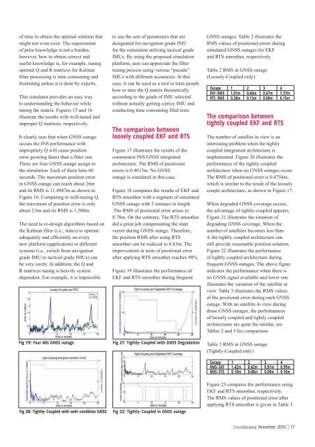
Figure 19 illustrates the performance of
EKF and RTS smoother during frequent
Fig 19: Four 60s GNSS outage Fig 21: Tightly-Coupled with GNSS Degradation
Fig 20: Tightly-Coupled with well-condition GNSS Fig 22: Tightly-Coupled in GNSS outage
GNSS outages. Table 2 illustrates the
RMS values of positional errors during
simulated GNSS outages for EKF
and RTS smoother, respectively.
Table 2 RMS in GNSS outage
(Loosely-Coupled only)
Outage 1 2 3 4
EKF-RMS 1.51m 0.66m 0.67m 1.37m
RTS_RMS 0.28m 0.13m 0.08m 0.15m
The comparison between
tightly coupled EKF and RTS
The number of satellite in view is an
interesting problem when the tightly
coupled integration architecture is
implemented. Figure 20 illustrates the
performance of the tightly coupled
architecture when no GNSS outages occur.
The RMS of positional error is 0.4754m,
which is similar to the result of the loosely
couple architecture, as shown in Figure 17.
When degraded GNSS coverage occurs,
the advantage of tightly-coupled appears.
Figure 21 illustrates the situation of
degrading GNSS coverage. When the
number of satellites becomes less than
4, the tightly coupled architecture can
still provide reasonable position solution.
Figure 22 illustrates the performance
of tightly coupled architecture during
frequent GNSS outages. The above figure
indicates the performance when there is
no GNSS signal available and lower one
illustrates the variation of the satellite in
view. Table 3 illustrates the RMS values
of the positional error during each GNSS
outage. With no satellite in view during
those GNSS outages, the performances
of loosely coupled and tightly coupled
architectures are quite the similar, see
Tables 2 and 3 for comparison.
Table 3 RMS in GNSS outage
(Tightly-Coupled only)
Outage 1 2 3 4
RMS-EKF 1.42m 0.42m 0.81m 0.99m
RMS-RTS 0.18m 0.08m 0.09m 0.10m
Figure 23 compares the performance using
EKF and RTS smoother, respectively.
The RMS values of positional error after
applying RTS smoother is given in Table 3.
Coordinates November 2010 | 17