Kaas. E., B. Sørensen, C. C. Tscherning, M. Veicherts Multi ...
Kaas. E., B. Sørensen, C. C. Tscherning, M. Veicherts Multi ...
Kaas. E., B. Sørensen, C. C. Tscherning, M. Veicherts Multi ...

Create successful ePaper yourself
Turn your PDF publications into a flip-book with our unique Google optimized e-Paper software.
{ C } , and s is the variance - covariances<br />
of the errors.<br />
where C = ij + s ij<br />
ij<br />
The estimate of the (M) parameters are obtained by<br />
The error-estimates and error-covariances, eckl are found with:<br />
H<br />
k<br />
T −1<br />
{ COV ( L , L ) } , NxM matrix<br />
= C<br />
k<br />
i<br />
~ T −1 −1 T −1<br />
X = ( A C A + W) ( A C y)<br />
2<br />
X<br />
T −1 −1<br />
m = ( A C A + W)<br />
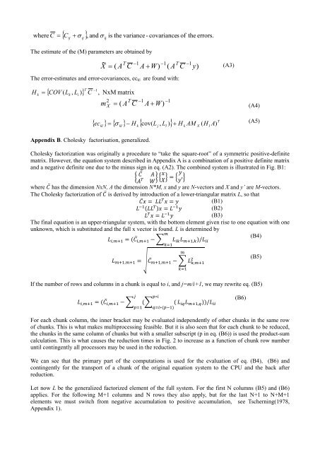
Appendix B. Cholesky factorisation, generalized.<br />
T<br />
{ ec } = { s<br />
} − H { cov( L , L ) } + H AM ( H A)<br />
kl<br />
kl<br />
Cholesky factorization was originally a procedure to “take the square-root” of a symmetric positive-definite<br />
matrix. However, the equation system described in Appendix A is a combination of a positive definite matrix<br />
and a negative definite one due to the minus sign in eq. (A2). The combined system is illustrated in Fig. B1: