Kaas. E., B. Sørensen, C. C. Tscherning, M. Veicherts Multi ...

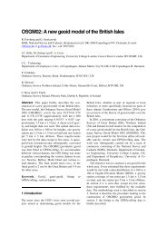
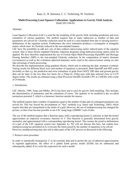
Abstract
Kaas. E., B. Sørensen, C. C. Tscherning, M. Veicherts
Multi-Processing Least Squares Collocation: Applications to Gravity Field Analysis.
Draft 2013-04-03
Least Squares Collocation (LSC) is used for the modeling of the gravity field, including prediction and error
estimation of various quantities. The method requires that as many unknowns as number of data and
parameters are solved for. Cholesky reduction must be used in a non-standard form due to missing positivedefiniteness
of the equation system. Furthermore the error estimation produces a rectangular or triangular
matrix which must be Cholesky reduced in the non-standard manner.
LSC have the possibility to add new sets of data without reprocessing earlier reduced parts of the equation
system. Due to these factors standard Cholesky reduction programs using multi-processing cannot easily be
applied. We have therefore implemented the use of Fortran Open Multi-Processing (OpenMP) and Message
Passing Interface (MPI) to the non-standard Cholesky reduction. In the computation of matrix elements
(covariances) as well as the evaluation spherical harmonic series used in the remove/restore setting we also
take advantage of multi-processing.
We describe the implementation using quadratic blocks, which aids in reducing the data transport overhead.
Timing results for different block sizes and number of equations is presented. Both OpenMP and MPI scales
favorably so that e.g. the prediction and error estimation of grids from GOCE TRF-data and ground gravity
data can be done in the less than two hours for a 25deg by 25deg area with data selected close to 0.125
degree nodes. The results are obtained using a Dual Processor Intel(R) Xeon(R) CPU at 2.40GHz with a total
of 24 threads.
1. Introduction.
LSC (Moritz, 1980, Torge and Müller, 2012) has been and is used for gravity field modeling. This includes
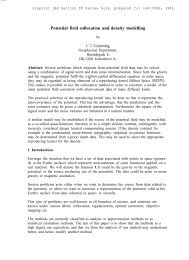
the determination of parameters and the estimation of errors. The quantity to be modeled is the so-called
anomalous potential T, which is a harmonic function outside the masses.
The method requires that a number of equations equal to the number of data and of contingent parameters are
solved for. This has forced the development of “fast” methods (e.g. Sansò and Tscherning, 2002) which
require that data are interpolated to the nodes of a grid. However, the use of multiprocessing has changed the
picture, so that it has become possible to use LSC using large (200000+) sets of data.
The use of the method requires that a function space with a reproducing kernel is selected, so that the kernel
approximates an empirical covariance function of T. This function is generally determined from gravity
anomalies and approximated with a corresponding reproducing kernel. This assures the positive-definiteness
of a part of the LSC equation system (see Appendix A). We will not discuss this here, but explain how
multiprocessing has permitted us to overcome the limits posed by the number of equations to be solved.
However, multiprocessing may also aid in other parts of the LSC process as discussed in the following.
2. Remove-store procedure.
In order to statistically homogenize T, to de-correlate data and to permit the use of spherical approximation
in regional applications, the effect of a global Earth gravity model (EGM) can be subtracted and
subsequently added. If we write the expression for such a model

Abstract
Kaas. E., B. Sørensen, C. C. Tscherning, M. Veicherts
Multi-Processing Least Squares Collocation: Applications to Gravity Field Analysis.
Draft 2013-04-03
Least Squares Collocation (LSC) is used for the modeling of the gravity field, including prediction and error
estimation of various quantities. The method requires that as many unknowns as number of data and
parameters are solved for. Cholesky reduction must be used in a non-standard form due to missing positivedefiniteness
of the equation system. Furthermore the error estimation produces a rectangular or triangular
matrix which must be Cholesky reduced in the non-standard manner.
LSC have the possibility to add new sets of data without reprocessing earlier reduced parts of the equation
system. Due to these factors standard Cholesky reduction programs using multi-processing cannot easily be
applied. We have therefore implemented the use of Fortran Open Multi-Processing (OpenMP) and Message
Passing Interface (MPI) to the non-standard Cholesky reduction. In the computation of matrix elements
(covariances) as well as the evaluation spherical harmonic series used in the remove/restore setting we also
take advantage of multi-processing.
We describe the implementation using quadratic blocks, which aids in reducing the data transport overhead.
Timing results for different block sizes and number of equations is presented. Both OpenMP and MPI scales
favorably so that e.g. the prediction and error estimation of grids from GOCE TRF-data and ground gravity
data can be done in the less than two hours for a 25deg by 25deg area with data selected close to 0.125
degree nodes. The results are obtained using a Dual Processor Intel(R) Xeon(R) CPU at 2.40GHz with a total
of 24 threads.
1. Introduction.
LSC (Moritz, 1980, Torge and Müller, 2012) has been and is used for gravity field modeling. This includes
the determination of parameters and the estimation of errors. The quantity to be modeled is the so-called
anomalous potential T, which is a harmonic function outside the masses.
The method requires that a number of equations equal to the number of data and of contingent parameters are
solved for. This has forced the development of “fast” methods (e.g. Sansò and Tscherning, 2002) which
require that data are interpolated to the nodes of a grid. However, the use of multiprocessing has changed the
picture, so that it has become possible to use LSC using large (200000+) sets of data.
The use of the method requires that a function space with a reproducing kernel is selected, so that the kernel
approximates an empirical covariance function of T. This function is generally determined from gravity
anomalies and approximated with a corresponding reproducing kernel. This assures the positive-definiteness
of a part of the LSC equation system (see Appendix A). We will not discuss this here, but explain how
multiprocessing has permitted us to overcome the limits posed by the number of equations to be solved.
However, multiprocessing may also aid in other parts of the LSC process as discussed in the following.
2. Remove-store procedure.
In order to statistically homogenize T, to de-correlate data and to permit the use of spherical approximation
in regional applications, the effect of a global Earth gravity model (EGM) can be subtracted and
subsequently added. If we write the expression for such a model

4. Reduction (factorization), solution of equations and error-estimation.
The LSC method has been applied since the 1960’ties on computers with very small central processing units
(CPU). Cholesky-reduction was used to reduce (not invert !) and solve the systems of equations. However
often it was possible to store elements of equation systems on external media like a disk or drum. A simple
implementation is described in (Poder and Tscherning, 1973) and used in the LSC implementation
(Tscherning, 1974). Here the equations were divided in rectangular blocks, filling in as many columns as
possible, and storing the blocks on an external media. However this implementation is not suitable for
multiprocessing, where each row may be processed individually using Cholesky-reduction, see Appendix B.
We therefore implemented a division of the matrices in square blocks called “chunks” like shown in Fig. (1).
Cholesky reduction is used in eq. (A2) with details in Appendix B. This is followed by what is known as
back-substitution and multiplication with the Cholesky-reduced in the other two equations, for details see
(Tscherning, 1980). However, the concatenated set of matrices is not positive definite, due to the “minus”
occurring in eq. (A2). This is however by-passed by using positive accumulation instead of negative
accumulation in the Cholesky-algorithm, see eq. (B4) and (B5). But for the use of multiprocessing this
causes difficulties, so that it is only used to reduce the chunks which do not contain a part of the A matrix.
This is also the primary reason for that standard LAPAC or similar equation solvers can not be used. Another
reason is that we want to be able to take advantage of the so-called permanency property (Freden, 1982),
where new columns can be added to an already reduced system of equations, and the reduction then
continued from the first chunk, which contains unreduced elements.
⎡c11
c12
c13
c14
c15
c16
c17
c18
c19
c110
⎤
⎢
⎥
⎢
0 c22
c23
c24
c25
c26
c27
c28
c29
c210
⎥
⎢ 0 0 c
⎥
33 c34
c35
c36
c37
c38
c39
c310
⎢
⎥
⎢ 0 0 0 c44
c45
c46
c47
c48
c49
c410
⎥
⎢ 0 0 0 0 c
⎥
55 c56
c57
c58
c59
c510
⎢
⎥
⎢ 0 0 0 0 0 c66
c67
c68
c69
c610
⎥
⎢ 0 0 0 0 0 0 c
⎥
77 c78
c79
c710
⎢
⎥
⎢ 0 0 0 0 0 0 0 c88
c89
c810
⎥
⎢
0 0 0 0 0 0 0 0 c
⎥
⎢
99 c910
⎥
⎢⎣
0 0 0 0 0 0 0 0 0 c1010
⎥⎦
Fig. 1. Chunk-wise division of the upper-triangular part of the

Fig. 2. Time for Cholesky reduction using 20 column block-size and 20 columns of blocks with 22
processors. Total number of observations 22464 with 22464/(20*20)+1 chunks.
The dependency of the number of processors and the chunk row number is clearly seen in Table 3. The time
used decreases when some processors are not in use, i.e. after the chunk row modulo number of processors
has become zero. However the time for transfer of a chunk to and from the CPU clearly also plays a role.
The pattern can easily be reproduced in a simulation, which a user should perform before embarking into a
major computation with many unknowns.
We see clearly that the smaller the chunks the faster the processing. There is however some system limits
which must be taken into account. Each chunk will be a separate file, and there will generally be an upper
limit for the number of files, which may be open at the same time.
Let N be the number of rows, and M the chunk-size, e.g. 400*400 as used in Fig. 2. For N=40000 we will
have NC=N/M, or 100 rows of chunks, i.e. (NC*(NC+1))/2 files in total. As may be easily shown, the
maximal number of open files is reached for chunk row number NC/2 and is equal to NC 2 /2, i.e. in this case
5000 open files.
5. Conclusion and outlook.
The use of multiprocessing has enabled the use of LSC for large sets of observations. The benefits are clearly
demonstrated when (1) the contribution of a spherical harmonic model is removed and restored, (2) when
establishing a column of covariances and (3) when factorizing the equation system. We have not yet finished
the implementation of MPI, using multiple computers in all 3 situations. But when this is done the plan is to
use up to 1 million data simultaneously.
References:
Arabelos, D. and C.C.Tscherning: Error-covariances of the estimates of spherical harmonic coefficients
computed by LSC, using second-order radial derivative functionals associated with realistic GOCE orbits.
J.Geodesy, DOI 10.1007/s00190-008-0250-9, 2008.
Forsberg, R. and C.C.Tscherning: An overview manual for the GRAVSOFT Geodetic Gravity Field
Modelling Programs. 2.edition. Contract report for JUPEM, 2008. Available as:
http://cct.gfy.ku.dk/publ_cct/cct1936.pdf

Freeden, W., 1982. On the Permanence Property in Spherical Spline Interpolation. Reports of the Department
of Geodetic Science and Surveying, No. 341, The Ohio State University, Columbus, Ohio.
Heiskanen, W.A. and H. Moritz: Physical Geodesy. W.H. Freeman & Co, San Francisco, 1967.
Moritz, H.: Advanced Physical Geodesy. H.Wichmann Verlag, Karlsruhe,1980.
Pavlis, N.K., S.A. Holmes, S.C. Kenyon, and J.K. Factor, An Earth Gravitational Model to Degree 2160:
EGM2008, presented at the 2008 General Assembly of the European Geosciences Union, Vienna, Austria,
April 13-18, 2008.
Poder, K. and C.C.Tscherning: Cholesky's Method on a Computer. The Danish Geodetic Institute Internal
Report No. 8, 1973.
Sansó, F. and C.C.Tscherning: Fast Spherical Collocation - Theory and Examples. J. of Geodesy, Vol. 77, pp.
101-112, DOI 10.1007/s00190-002-0310-5,
2003.
Tscherning, C.C.: A FORTRAN IV Program for the Determination of the Anomalous Potential Using
Stepwise Least Squares Collocation. Reports of the Department of Geodetic Science No. 212, The Ohio State
University, Columbus, Ohio, 1974.
Tscherning, C.C.: A Users Guide to Geopotential Approximation by Stepwise Collocation on the RC 4000-
Computer. Geodaetisk Institut Meddelelse No. 53, 1978.
Tscherning, C.C. and K.Poder: Some Geodetic applications of Clenshaw Summation. Bolletino di Geodesia
e Scienze Affini, Vol. XLI, no. 4,pp. 349-375, 1982.
Tscherning, C.C. and M.Veicherts: Accelerating generalized Cholesky decomposition using multiple
processors. Power point presentation, 2008. Available as http://cct.gfy.ku.dk/publ_cct/accelerating08.ppt
Appendix A: Basic equations (cf. Heiskanen and Moritz, 1967 and Moritz 1980).
The gravity potential W, is the sum of the potential V due to the attraction of the masses and the centrifugal
potential. The anomalous potential is the difference between W and the normal potential U. In space
quantities related to V are measured, while at the surface of the Earth W is the important quantity. T is
however the same everywhere, because the centrifugal part is eliminated.
T may be represented by a series in spherical harmonics, cf. eq. (1).
The basic observation equation for LSC is
y
T
= L ( T ) + e + A X , (A1)
i i LSC i i
where yi is a vector of n observations, Li is a vector of functionals associating T with the observarion, ei is a

{ C } , and s is the variance - covariances
of the errors.
where C = ij + s ij
ij
The estimate of the (M) parameters are obtained by
The error-estimates and error-covariances, eckl are found with:
H
k
T −1
{ COV ( L , L ) } , NxM matrix
= C
k
i
~ T −1 −1 T −1
X = ( A C A + W) ( A C y)
2
X
T −1 −1
m = ( A C A + W)
Appendix B. Cholesky factorisation, generalized.
T
{ ec } = { s
} − H { cov( L , L ) } + H AM ( H A)
kl
kl
Cholesky factorization was originally a procedure to “take the square-root” of a symmetric positive-definite
matrix. However, the equation system described in Appendix A is a combination of a positive definite matrix
and a negative definite one due to the minus sign in eq. (A2). The combined system is illustrated in Fig. B1:

The calculation of error-estimates for several quantities (R) may also take advantage of this. Let P be an
(N+M)*R matrix of covariances between the observations and the R quantities to be predicted and Q an RxR
matrix of covariances of the quantities to be predicted. Then we have an extended system