Probability Density Estimation using Isocontours and Isosurfaces ...
Probability Density Estimation using Isocontours and Isosurfaces ...
Probability Density Estimation using Isocontours and Isosurfaces ...
You also want an ePaper? Increase the reach of your titles
YUMPU automatically turns print PDFs into web optimized ePapers that Google loves.
isocontours at intensity levels that are infinitesimally apart. We<br />
extended the idea to the case of joint density between two<br />
images, both in 2D <strong>and</strong> 3D, as also the case of multiple images<br />
in 2D. Empirically, we showed superior noise resistance on<br />
registration experiments involving rotations <strong>and</strong> affine transformations.<br />
Furthermore, we also suggested a faster, biased alternative<br />
based on counting pixel intersections which performs well, <strong>and</strong><br />
extended the method to h<strong>and</strong>le volume datasets. The relationship<br />
between our techniques <strong>and</strong> histogramming with multiple subpixel<br />
samples was also discussed. Here are a few clarifications<br />
about our technique in question/answer format.<br />
(1) How does our method compare to histogramming on<br />
an up-sampled image?<br />
If an image is up-sampled several times <strong>and</strong> histogramming is<br />
performed on it, there will be more samples for the histogram. At<br />
a theoretical level, though, there is still the issue of not being able<br />
to relate the number of bins to the available number of samples.<br />
Furthermore, it is recommended that the rate of increase in the<br />
number of bins be less than the square root of the number of<br />
samples for computing the joint density between two images [35],<br />
[8]. If there are d images in all, the number of bins ought to be<br />
less than N 1 d , where N is the total number of pixels, or samples<br />
to be taken [35], [8]. Consider that this criterion suggested that N<br />
samples were enough for a joint density between two images with<br />
χ bins. Suppose that we now wished to compute a joint density<br />
with χ bins for d images of the same size. This would require<br />
the images to be up-sampled by a factor of at least N d−2<br />
2 , which<br />
is exponential in the number of images. Our simple area-based<br />
method clearly avoids this problem.<br />
(2) How does one choose the optimal number of bins or<br />
the optimal interpolant for our method?<br />
One can choose as many bins as needed for the application,<br />
constrained only by availability of appropriate hardware (processor<br />
speed or memory). We chose a (piece-wise) linear interpolant<br />
for the sake of simplicity, though in principle any other interpolant<br />
could be used. It is true that we are making an assumption on<br />
the continuity of the intensity function which may be violated<br />
in natural images. However, given a good enough resolution<br />
of the input image, interpolation across a discontinuity will<br />
have a negligible impact on the density as those discontinuities<br />
are essentially a measure zero set. One could even incorporate<br />
an edge-preserving interpolant [20] by running an anisotropic<br />
diffusion to detect the discontinuities <strong>and</strong> then taking care not<br />
to interpolate across the two sides of an edge.<br />
(3) What are the limitations of our technique?<br />
As of now, our technique is not differentiable, which is<br />
important for non-rigid registration. Differentiability could be<br />
achieved by fitting (say) a spline to the obtained probability tables.<br />
However, this again requires smoothing the density estimate in<br />
a manner that is not tied to the image geometry. Hence, this<br />
goes against the philosophy of our approach. For practical or<br />
empirical reasons, however, there is no reason why one should<br />
not experiment with this.<br />
(4) Other avenues for future research:<br />
Currently, we do not have a closed form expression for our<br />
density estimate. Expressing the marginal <strong>and</strong> joint densities<br />
solely in terms of the parameters of the chosen image interpolant<br />
is a challenging theoretical problem. We could also apply our<br />
density estimation scheme to images whose pixel values belong<br />
to a non-Euclidean manifold, such as unit vectors or covariance<br />
matrices, or to data fields that are defined on non-Euclidean<br />
surfaces.<br />
APPENDIX<br />
In this section, we derive the expression for the marginal density<br />
of the intensity of a single 2D image. We begin with Eq. (4)<br />
derived in Section II-A:<br />
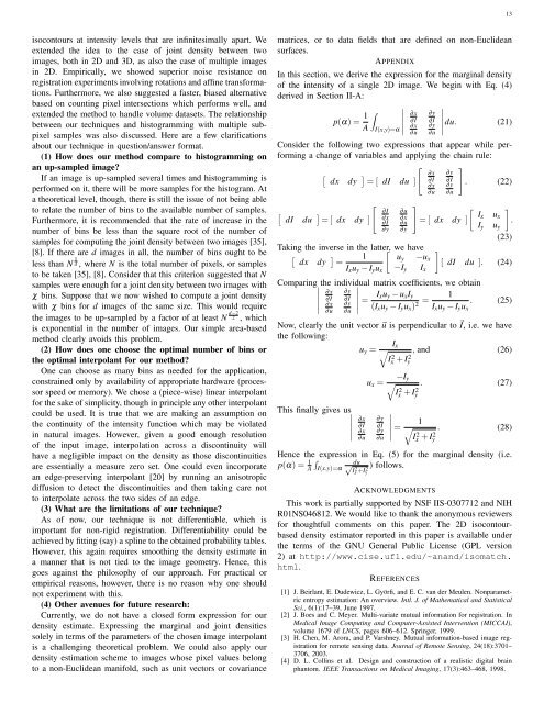
p(α) = 1<br />
<br />
A<br />
I(x,y)=α<br />
<br />
<br />
<br />
<br />
<br />
∂x<br />
∂I<br />
∂x<br />
∂u<br />
∂y<br />
∂I<br />
∂y<br />
∂u<br />
13<br />
<br />
<br />
<br />
du.<br />
(21)<br />
<br />
Consider the following two expressions that appear while performing<br />
a change of variables <strong>and</strong> applying the chain rule:<br />
<br />
∂x ∂y<br />
dx dy = [ dI du ] ∂I ∂I . (22)<br />
dI du = [ dx dy ]<br />
<br />
∂I<br />
∂x<br />
∂I<br />
∂y<br />
∂u<br />
∂x<br />
∂u<br />
∂y<br />
Taking the inverse in the latter, we have<br />
1 uy −ux<br />
dx dy =<br />
−Iy Ix<br />
Ixuy − Iyux<br />
<br />
∂x<br />
∂u<br />
∂y<br />
∂u<br />
<br />
Ix ux<br />
= [ dx dy ]<br />
Iy uy<br />
<br />
.<br />
(23)<br />
<br />
[ dI du ]. (24)<br />
Comparingthe individual matrix coefficients, we obtain<br />
∂x ∂y <br />
<br />
∂I ∂I <br />
<br />
= Ixuy − uxIy 1<br />
= . (25)<br />
(Ixuy − Iyux) 2<br />
∂x<br />
∂u<br />
∂y<br />
∂u<br />
Ixuy − Iyux<br />
Now, clearly the unit vector u is perpendicular to I, i.e. we have<br />
the following:<br />
This finally gives us <br />
uy =<br />
∂x<br />
∂I<br />
∂x<br />
∂u<br />
Ix<br />
<br />
I 2 x + I 2 y<br />
, <strong>and</strong> (26)<br />
ux = −Iy<br />
<br />
I2 x + I2 . (27)<br />
y<br />
∂y<br />
∂I<br />
∂y<br />
∂u<br />
<br />
<br />
<br />
<br />
=<br />
1<br />
<br />
I2 x + I2 . (28)<br />
y<br />
Hence the expression in Eq. (5) for the marginal density (i.e.<br />
p(α) = 1 <br />
du<br />
A I(x,y)=α ) follows.<br />
√ I 2 x +I 2 y<br />
ACKNOWLEDGMENTS<br />
This work is partially supported by NSF IIS-0307712 <strong>and</strong> NIH<br />
R01NS046812. We would like to thank the anonymous reviewers<br />
for thoughtful comments on this paper. The 2D isocontourbased<br />
density estimator reported in this paper is available under<br />
the terms of the GNU General Public License (GPL version<br />
2) at http://www.cise.ufl.edu/~an<strong>and</strong>/isomatch.<br />
html.<br />
REFERENCES<br />
[1] J. Beirlant, E. Dudewicz, L. Györfi, <strong>and</strong> E. C. van der Meulen. Nonparametric<br />
entropy estimation: An overview. Intl. J. of Mathematical <strong>and</strong> Statistical<br />
Sci., 6(1):17–39, June 1997.<br />
[2] J. Boes <strong>and</strong> C. Meyer. Multi-variate mutual information for registration. In<br />
Medical Image Computing <strong>and</strong> Computer-Assisted Intervention (MICCAI),<br />
volume 1679 of LNCS, pages 606–612. Springer, 1999.<br />
[3] H. Chen, M. Arora, <strong>and</strong> P. Varshney. Mutual information-based image registration<br />
for remote sensing data. Journal of Remote Sensing, 24(18):3701–<br />
3706, 2003.<br />
[4] D. L. Collins et al. Design <strong>and</strong> construction of a realistic digital brain<br />
phantom. IEEE Transactions on Medical Imaging, 17(3):463–468, 1998.


