Probability Density Estimation using Isocontours and Isosurfaces ...

Hence, we have
p(α) = 1
d
A dα
I(x,y)≤α
dxdy. (3)
We can now adopt a change of variables from the spatial
coordinates (x,y) to u(x,y) and I(x,y), where u and I are the
directions parallel and perpendicular to the level curve of intensity
α, respectively. Observe that I points in the direction of the image
gradient, or the direction of maximum intensity change. Noting
this fact, we now obtain the following:
p(α) = 1
A
I(x,y)=α
∂x
∂I
∂x
∂u
∂y
∂I
∂y
∂u
du.
(4)
Note that in Eq. (4), dα and dI have “canceled” each other out,
as they both stand for intensity change. Upon a series of algebraic
manipulations, we are now left with the following expression
for p(α) (with a more detailed derivation to be found in the
Appendix):
p(α) = 1
A I(x,y)=α
du
( ∂I
∂x )2 + ( ∂I
∂y )2
. (5)
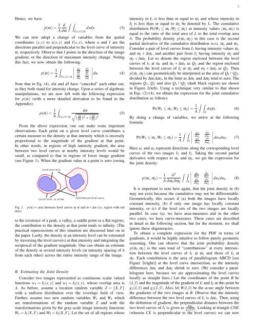
From the above expression, one can make some important
observations. Each point on a given level curve contributes a
certain measure to the density at that intensity which is inversely
proportional to the magnitude of the gradient at that point.
In other words, in regions of high intensity gradient, the area
between two level curves at nearby intensity levels would be
small, as compared to that in regions of lower image gradient
(see Figure 1). When the gradient value at a point is zero (owing
Level curve at α
Level Curve at α+∆α
Area between level curves
Fig. 1. p(α) ∝ area between level curves at α and α + ∆α (i.e. region with red
dots)
to the existence of a peak, a valley, a saddle point or a flat region),
the contribution to the density at that point tends to infinity. (The
practical repercussions of this situation are discussed later on in
the paper. Lastly, the density at an intensity level can be estimated
by traversing the level curve(s) at that intensity and integrating the
reciprocal of the gradient magnitude. One can obtain an estimate
of the density at several intensity levels (at intensity spacing of h
from each other) across the entire intensity range of the image.
B. Estimating the Joint Density
Consider two images represented as continuous scalar valued
functions w1 = I1(x,y) and w2 = I2(x,y), whose overlap area is
A. As before, assume a location random variable Z = {X,Y }
with a uniform distribution over the (overlap) field of view.
Further, assume two new random variables W1 and W2 which
are transformations of the random variable Z and with the
transformations given by the gray-scale image intensity functions
W1 = I1(X,Y ) and W2 = I2(X,Y ). Let the set of all regions whose
intensity in I1 is less than or equal to α1 and whose intensity in
I2 is less than or equal to α2 be denoted by L. The cumulative
distribution Pr(W1 ≤ α1,W2 ≤ α2) at intensity values (α1,α2) is
equal to the ratio of the total area of L to the total overlap area
A. The probability density p(α1,α2) in this case is the second
partial derivative of the cumulative distribution w.r.t. α1 and α2.
Consider a pair of level curves from I1 having intensity values α1
and α1 + ∆α1, and another pair from I2 having intensity α2 and
α2 + ∆α2. Let us denote the region enclosed between the level
curves of I1 at α1 and α1 + ∆α1 as Q1 and the region enclosed
between the level curves of I2 at α2 and α2 + ∆α2 as Q2. Then
p(α1,α2) can geometrically be interpreted as the area of Q1 ∩Q2,
divided by ∆α1∆α2, in the limit as ∆α1 and ∆α2 tend to zero. The
regions Q1, Q2 and also Q1 ∩ Q2 (dark black region) are shown
in Figure 2(left). Using a technique very similar to that shown
in Eqs. (2)-(4), we obtain the expression for the joint cumulative
distribution as follows:
Pr(W1 ≤ α1,W2 ≤ α2) = 1
A
L
3
dxdy. (6)
By doing a change of variables, we arrive at the following
formula:
Pr(W1 ≤ α1,W2 ≤ α2) = 1
A L
∂x
∂u1
∂x
∂u2
∂y
∂u1
∂y
∂u2
du1du2. (7)
Here u1 and u2 represent directions along the corresponding level
curves of the two images I1 and I2. Taking the second partial
derivative with respect to α1 and α2, we get the expression for
the joint density:
p(α1,α2) = 1 ∂
A
2
∂α1∂α2 L
∂x
∂u1
∂x
∂u2
∂y
∂u1
∂y
∂u2
du1du2. (8)
It is important to note here again, that the joint density in (8)
may not exist because the cumulative may not be differentiable.
Geometrically, this occurs if (a) both the images have locally
constant intensity, (b) if only one image has locally constant
intensity, or (c) if the level sets of the two images are locally
parallel. In case (a), we have area-measures and in the other
two cases, we have curve-measures. These cases are described
in detail in the following section, but for the moment, we shall
ignore these degeneracies.
To obtain a complete expression for the PDF in terms of
gradients, it would be highly intuitive to follow purely geometric
reasoning. One can observe that the joint probability density
p(α1,α2) is the sum total of “contributions” at every intersection
between the level curves of I1 at α1 and those of I2 at
α2. Each contribution is the area of parallelogram ABCD [see
Figure 2(right)] at the level curve intersection, as the intensity
differences ∆α1 and ∆α2 shrink to zero. (We consider a parallelogram
here, because we are approximating the level curves
locally as straight lines.) Let the coordinates of the point B be
( ˜x, ˜y) and the magnitude of the gradient of I1 and I2 at this point be
g1( ˜x, ˜y) and g2( ˜x, ˜y). Also, let θ( ˜x, ˜y) be the acute angle between
the gradients of the two images at B. Observe that the intensity
difference between the two level curves of I1 is ∆α1. Then, using
the definition of gradient, the perpendicular distance between the
two level curves of I1 is given as ∆α1
g1( ˜x, ˜y) . Looking at triangle CDE
(wherein CE is perpendicular to the level curves) we can now