Probability Density Estimation using Isocontours and Isosurfaces ...

Center of
voxel
Center of
voxel
(a)
(b)
Face of one of
the tetrahedra
Each square face is the base
of four tetrahedra
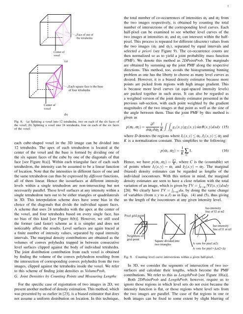
Fig. 8. (a) Splitting a voxel into 12 tetrahedra, two on each of the six faces of
the voxel; (b) Splitting a voxel into 24 tetrahedra, four on each of the six faces
of the voxel.
each cube-shaped voxel in the 3D image can be divided into
12 tetrahedra. The apex of each tetrahedron is located at the
center of the voxel and the base is formed by dividing one of
the six square faces of the cube by one of the diagonals of that
face [see Figure 8(a)]. Within each triangular face of each such
tetrahedron, the intensity can be assumed to be a linear function
of location. Note that the intensities in different faces of one and
the same tetrahedron can thus be expressed by different functions,
all of them linear. Hence the isosurfaces at different intensity
levels within a single tetrahedron are non-intersecting but not
necessarily parallel. These level surfaces at any intensity within a
single tetrahedron turn out to be either triangles or quadrilaterals
in 3D. This interpolation scheme does have some bias in the
choice of the diagonals that divide the individual square faces.
A scheme that uses 24 tetrahedra with the apex at the center of
the voxel, and four tetrahedra based on every single face, has
no bias of this kind [see Figure 8(b)]. However, we still used
the former (and faster) scheme as it is simpler and does not
noticeably affect the results. Level surfaces are again traced at
a finite number of intensity values, separated by equal intensity
intervals. The marginal density contributions are obtained as the
volumes of convex polyhedra trapped in between consecutive
level surfaces clipped against the body of individual tetrahedra.
The joint distribution contribution from each voxel is obtained
by finding the volume of the convex polyhedron resulting from
the intersection of corresponding convex polyhedra from the two
images, clipped against the tetrahedra inside the voxel. We refer
to this scheme of finding joint densities as VolumeProb.
G. Joint Densities by Counting Points and Measuring Lengths
For the specific case of registration of two images in 2D, we
present another method of density estimation. This method, which
was presented by us earlier in [23], is a biased estimator that does
not assume a uniform distribution on location. In this technique,
the total number of co-occurrences of intensities α1 and α2 from
the two images respectively, is obtained by counting the total
number of intersections of the corresponding level curves. Each
half-pixel can be examined to see whether level curves of the
two images at intensities α1 and α2 can intersect within the halfpixel.
This process is repeated for different (discrete) values from
the two images (α1 and α2), separated by equal intervals and
selected a priori (see Figure 9). The co-occurrence counts are
then normalized so as to yield a joint probability mass function
(PMF). We denote this method as 2DPointProb. The marginals
are obtained by summing up the joint PMF along the respective
directions. This method, too, avoids the histogramming binning
problem as one has the liberty to choose as many level curves as
desired. However, it is a biased density estimator because more
points are picked from regions with high image gradient. This
is because more level curves (at equi-spaced intensity levels)
are packed together in such areas. It can also be regarded as
a weighted version of the joint density estimator presented in the
previous sub-section, with each point weighted by the gradient
magnitudes of the two images at that point as well as the sine of
the angle between them. Thus the joint PMF by this method is
given as
∂ 2
1
p(α1,α2) = g1(x,y)g2(x,y)sinθ(x,y)dxdy (15)
∂α1∂α2 K D
where D denotes the regions where I1(x,y) ≤ α1,I2(x,y) ≤ α2 and
K is a normalization constant. This simplifies to the following:
p(α1,α2) = 1
K ∑1. (16)
C
Hence, we have p(α1,α2) = |C|
K , where C is the (countable) set
of points where I1(x,y) = α1 and I2(x,y) = α2. The marginal
(biased) density estimates can be regarded as lengths of the
individual isocontours. With this notion in mind, the marginal
density estimates are seen to have a close relation with the total
variation of an image, which is given by TV =
I=α |∇I(x,y)|dxdy
[26]. We clearly have TV =
I=α du, by doing the same change
of variables (from x,y to u,I) as in Eqs. (4) and (5), thus giving
us the length of the isocontours at any given intensity level.
Pixel grid point
Neighbors of
grid point
Square divided into
two triangles
Iso-intensity
line of I2 at α2
A vote for p(α1,α2)
7
Iso-intensity
line of I1 at α1
A vote for p(α1+∆,α2+∆)
Fig. 9. Counting level curve intersections within a given half-pixel.
In 3D, we consider the segments of intersection of two isosurfaces
and calculate their lengths, which become the PMF
contributions. We refer to this as LengthProb [see Figure 10(a)].
Both 2DPointProb and LengthProb, however, require us to
ignore those regions in which level sets do not exist because the
intensity function is flat, or those regions where level sets from
the two images are parallel. The case of flat regions in one or
both images can be fixed to some extent by slight blurring of