Scalar Transport - Turbulence Mechanics/CFD Group

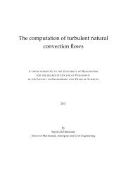
School of Mechanical Aerospace and Civil Engineering 

TPFE MSc Advanced Turbulence Modelling 

Scalar Transport 

T. J. Craft 

George Begg Building, C41 

Reading: 

S. Pope, Turbulent Flows 

D. Wilcox, Turbulence Modelling for CFD 

Closure Strategies for Turbulent and Transitional 

Flows, (Eds. B.E. Launder, N.D. Sandham) 

Notes: Blackboard and CFD/TM web server: 

http://cfd.mace.manchester.ac.uk/tmcfd 

- People - T. Craft - Online Teaching Material 

Scalar Transport 2011/12 1 / 18 

◮ Equation (1) can be averaged in the same way as the momentum 

equations. First, we split Φ into mean and fluctuating parts: 

Φ(x,t) = Φ(x) + φ(x,t) (2) 

◮ Substituting into equation (1) and averaging leads to an equation of the 

form 

∂Φ ∂ 

+ UjΦ 

∂t ∂xj = ∂ 

 

λ 

∂xj ∂Φ 

 

− u 

∂x 

jφ + 

j 

SΦ 

(3) 

where SΦ represents the averaged source terms from the original 

instantaneous equation. 

◮ Comparing with the Reynolds averaged Navier-Stokes equations, in this 

case the additional terms involve the turbulent scalar fluxes, u jφ. 

◮ In order to close the equation, we need to devise models for these 

turbulent scalar fluxes. 

◮ For simplicity, we consider the problem of modelling turbulent heat fluxes, 

uiθ, although the principles are easily extended to other scalars. 


Introduction 

◮ In many CFD applications we may be interested in predicting the 

behaviour of scalar quantities such as enthalpy, temperature, mass 

fraction of a chemical species, etc. 

◮ Consider a property Φ transported by the flow. We assume that its 

evolution can be described by the equation 

∂ 

Φ 

∂t 

∂ 

 

+ Uj Φ 

= 

∂xj ∂ 

∂xj λ ∂ 

Φ 

+ 

∂xj SΦ 

where SΦ represents any source or sink term that may be present. 

◮ If Φ is enthalpy or temperature, the flow is low speed and the effects of 

viscous heating are negligible, then SΦ can often be ignored. 

◮ If Φ represents the mass fraction of a species being consumed or 

produced by chemical reaction, then SΦ may be of great importance and 

has to be modelled from the details of the reaction process. 

◮ If Φ represents temperature, then λ is simply ν/Pr where Pr is the 

molecular Prandtl number of the fluid. 


Eddy-Diffusivity Modelling 

◮ A linear eddy-viscosity model approximates the turbulent stresses by: 

 

∂Ui 

uiuj = (2/3)kδij − νt + 

∂xj ∂U 

j 

(4) 

∂xi ◮ An obvious extension of this is to introduce an eddy-diffusivity for the 

scalar fluxes, related to the turbulent viscosity: 

u iθ = − νt 

σt 

∂Θ 

∂x i 

◮ The total flux terms in the mean temperature transport equation then 

become 

 

∂ ν νt ∂Θ 

+ 

Pr σt 

∂x k 

◮ The turbulent Prandtl number, σt, is often assumed to be constant. 

◮ In a near-wall flow, σt = 0.9 is usually adopted. However, in free flows a 

lower value (around 0.7) is more appropriate. 


∂x k 

(1) 

(5)

Scalar Fluxes in Simple Shear 

◮ An exact equation can be derived for u iθ, which shows it has a 

generation term of the form 

P iθ = −u iu k 

∂Θ 

− u 

∂x 

kθ 

k 

∂Ui ∂xk ◮ In simple shear flow U = U(y), Θ = Θ(y), this gives: 

P1θ = −uv dΘ 

dy 

dΘ 

P2θ = −v 2 

dy 

− vθ dU 

dy 

◮ This suggests both the wall-normal and wall-parallel scalar fluxes will be 

non-zero. 

◮ Measurements and DNS data show that generally |uθ | > |vθ |, 

particularly in the near-wall region. 


◮ However, the eddy diffusivity model gives: 

vθ = − νt dΘ 

σt dy 

U(y) 

and uθ = 0 

ie. zero turbulent scalar flux in the streamwise direction. 

◮ Making the usual boundary layer approximations, the (steady) mean 

scalar transport equation becomes 

U ∂Θ 

 

∂Θ ∂ 

+ V = α 

∂x ∂y ∂y 

∂Θ 

 

− vθ 

∂y 

◮ Consequently, if streamwise gradients are small compared to 

cross-stream ones, the above error in uθ may not have serious 

consequences. 

◮ However, the error may be more serious in buoyancy-influenced or other 

complex flows. 


y 

x 

Θ(y) 

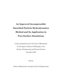
Homogeneous Shear Flow 

y 

x 

U(y) 

Θ(y) 

Expts: Tavoularis & Corrsin (1981) 

y 

x 

Chevray & Tutu (1978) 

Expts: 

q 

U(y) 

T(y) 

q 

Heated Plane Channel 

y x 

DNS: Horiuti (1992) 

Heated Axisymmetric Jet 


Generalized Gradient Diffusion Modelling 

◮ A somewhat better model for the scalar fluxes arises from the Daly & 

Harlow (1970) Generalised Gradient Diffusion Hypothesis (GGDH): 

◮ In a simple shear flow this gives 

k dΘ 

vθ = −cθ v 2 

ε dy 

k 

uiθ = −cθ 

ε u ∂Θ 

iuj ∂xj k dΘ 

and uθ = −cθ uv 

ε dy 

◮ This does at least give a non-zero uθ, and also better reflects the 

dependence of vθ on v 2 , seen in the generation terms. 

◮ If a stress transport model or non-linear EVM is used which gives good 

stress anisotropy levels, the above form can be used as is (typically with 

a coefficient cθ around 0.3). 

Scalar Transport 2011/12 8 / 18

◮ With an EVM (which will not generally provide good normal stress 

predictions), the GGDH can still be used with some modification. 

◮ Ince & Launder (1989) used this model in conjunction with a linear 

eddy-viscosity model for the stresses, taking cθ = (3/2)(cμ/σt). 

◮ In a shear flow (where the model returns v 2 = (2/3)k) this gives 

k dΘ cμ k 

vθ = −cθ v 2 = − 

ε dy σt 

2 dΘ 

ε dy 

k dΘ 

uθ = −cθ uv 

ε dy 

which gives vθ as in the eddy-diffusivity model, but should give a better 

approximation of uθ. 

◮ More complex algebraic scalar flux models have been proposed, some 

developed along similar routes to the non-linear eddy-viscosity models 

examined earlier for the Reynolds stresses. 


◮ Density fluctuations are often expressed in terms of temperature 

fluctuations, by introducing the thermal expansion coefficient: 

β = − 1 ∂ρ 

ρ ∂Θ 

◮ The buoyancy source term in the k equation then becomes 

(9) 

G k = −β g i u iθ (10) 

◮ Note that the buoyant generation of k depends on the turbulent scalar 

fluxes. 

◮ Depending on the sign of vθ, buoyancy can either enhance or reduce k 

levels: 

◮ In a stably stratified layer (with dΘ/dy > 0) we would typically have 

vθ < 0 and hence (with g2 < 0), G k is negative. 

◮ In an unstable layer, dΘ/dy < 0, and hence vθ > 0 and G k is 

positive. 


Buoyancy Effects 

◮ One important application where temperature (or concentration) 

differences must be properly accounted for is in buoyancy-affected flows. 

◮ In that case, there is an additional source term in the momentum 

equation: 

D(ρUi) 

Dt = ... + ρg i (6) 

◮ This results in an additional term in the transport equation for the 

fluctuating velocity: 

Du i 

Dt = ... + ρ′ g i/ρ (7) 

where ρ ′ is the fluctuating density. 

◮ Consequently, one gets an additional generation term in the turbulent 

kinetic energy equation: 

G k = (1/ρ)g i u iρ ′ (8) 


Buoyancy in Stress Transport Models 

◮ The buoyancy-related term appearing in the transport equation for u i 

leads to an additional generation term in the stress transport equations: 

where 

Du iu j 

Dt = P ij + G ij + φ ij − ε ij + d ij (11) 

G ij = −β g i u jθ − β g j u iθ (12) 

◮ When modelling the pressure-strain redistribution process, a contribution 

due to buoyancy should also be included: 

φ ij = φ ij1 + φ ij2 + φ ij3 

◮ Within the framework of the modelling adopted earlier, φ ij3 is 

approximated in a similar manner to φ ij2: 

(13) 

φ ij3 = −c3(G ij − (1/3)G kkδ ij) (14) 

◮ φ ij3 is thus assumed to redistribute the buoyancy generation. 


◮ In some instances it may be sufficient to model the scalar fluxes u iθ 

using a GGDH approach (or similar) as described earlier. 

◮ However, in strongly buoyant flows this may not be adequate, since the 

scalar fluxes are themselves affected by buoyancy. 

◮ Some extended algebraic heat flux models have been proposed, 

incorporating some buoyancy effects (eg. Hanjalić et al, 1996). 

◮ Another option is to adopt a full second-moment closure, solving 

transport equations for the scalar fluxes also. 

◮ Scalar flux transport equations can be derived in a similar manner to 

those for the Reynolds stresses. The result can be written in the form 

Du iθ 

Dt = Piθ + Giθ + φiθ − εiθ + diθ (15) 

◮ The generation terms P iθ and G iθ are exact: 

P iθ = −u iu k 

∂Θ 

− u 

∂x 

kθ 

k 

∂Ui ∂xk (16) 

G iθ = −β g i θ 2 (17) 


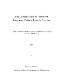
Negatively-Buoyant Jet 

◮ Axisymmetric downward 

directed buoyant jet. 

◮ Experiment of Cresswell et al 

(1989). 

◮ Velocity and shear stress 

profiles one diameter 

downstream of jet discharge. 

—— TCL RSM; – – Basic RSM 


◮ Other terms in the transport equation have to be modelled. 

◮ Similar assumptions are typically made for these as for the corresponding 

terms in the stress transport equations. However, the details will not be 

covered in this course. 

◮ The scalar flux buoyancy generation depends on the scalar variance, θ 2 . 

◮ This can be obtained by solving its transport equation, of the form 

where the generation rate is given by 

Dθ 2 

Dt = Pθ − 2εθ + diffusion (18) 

Pθ = −2u iθ ∂Θ 

◮ The dissipation rate εθ is usually either modelled algebraically by 

assuming that thermal and dynamic timescales are related (eg. 

R = (k/ε)(2εθ /θ 2 ) being constant), or obtained from its own modelled 

transport equation. 


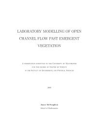
Opposed/Buoyant Wall Jet 

∂xi 

◮ Isothermal and buoyant cases studied. 

◮ LES data from Addad et al (2004). 

◮ Requires a good outer flow and near-wall 

modelling for accuracy. 

◮ Vertical 

velocity 

contours. 


Stably Stratified Mixing Layer 

◮ Studied experimentally by 

Uittenbogaard (1998). 

◮ U1 = 0.5m/s, ρ1 = 1015kg/m 3 

◮ U2 = 0.3m/s, ρ2 = 1030kg/m 3 

◮ Linear k-ε scheme overpredicts 

turbulence levels and hence mixing. 

◮ Second-moment closures do better at 

capturing buoyancy effects on scalar 

fluxes and hence reduce mixing. 

◮ In this case, as turbulence levels 

decrease, modelling of diffusion 

becomes more influential. 


References 

◮ Addad, Y., Benhamadouche, S., Laurence, D., (2004) The negatively buoyant jet: LES 

results, Int. J. Heat and Fluid Flow, vol. 25, pp. 795-808. 

◮ Chevray, R., Tutu, N.K., (1978) Intermittency and preferential transport of heat in a round jet, 

J. Fluid Mech., vol. 88, p. 133. 

◮ Cresswell, R., Haroutunian, V., Ince, N.Z., Launder, B.E., Szczepura, R.T., (1989) 

Measurement and modelling of buoyancy-modified elliptic turbulent shear flows, Proc. 7th 

Turbulent Shear Flows Symposium, Stanford University. 

◮ Daly, B.J., Harlow, F.H., (1970) Transport equations in turbulence, Phys. Fluids, vol. 13, pp. 

2634-2649. 

◮ Hanjalić, K., Kenjeres, S., Durst, F., (1996) Natural convection in partitioned two-dimensional 

enclosures at higher Rayleigh numbers, Int. J. Heat Mass Transfer, vol. 39, pp. 1407-1427. 

◮ Horiuti, K., (1992) Assessment of two-equation models of turbulent passive-scalar diffusion 

in channel flow, J. Fluid Mech., vol. 238, pp. 405-433. 

◮ Ince, N.Z., Launder, B.E., (1989) On the computation of buoyancy-driven turbulent flow in 

rectangular enclosures, Int. J. Heat Fluid Flow, vol. 10, pp. 110-117. 

◮ Tavoularis, S., Corrsin, S., (1981) Experiments in nearly homogeneous turbulent shear flow 

with a uniform mean temperature gradient. Part 1., J. Fluid Mech., vol. 104, pp. 311-347. 

◮ Uittenbogaard, R.E., (1998) Measurement of turbulence fluxes in a steady, stratified, mixing 

layer, Proc. 3rd Int. Symposium on Refined Flow Modelling and Turbulence Measurements, 

Tokyo.

Scalar Transport - Turbulence Mechanics/CFD Group

Create successful ePaper yourself

Delete template?

Save as template?