Lecture 3: A Brief Overview of Molecular Phylogeny - MCD Biology
Lecture 3: A Brief Overview of Molecular Phylogeny - MCD Biology
Lecture 3: A Brief Overview of Molecular Phylogeny - MCD Biology
Create successful ePaper yourself
Turn your PDF publications into a flip-book with our unique Google optimized e-Paper software.
1<br />
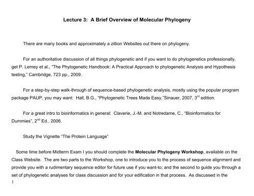
<strong>Lecture</strong> 3: A <strong>Brief</strong> <strong>Overview</strong> <strong>of</strong> <strong>Molecular</strong> <strong>Phylogeny</strong><br />
There are many books and approximately a zillion Websites out there on phylogeny.<br />
For an authoritative discussion <strong>of</strong> all things phylogenetic and if you want to do phylogenetics pr<strong>of</strong>essionally,<br />
get P. Lemey et al., “The Phylogenetic Handbook: A Practical Approach to phylogenetic Analysis and Hypothesis<br />
testing,” Cambridge, 723 pp., 2009.<br />
For a step-by-step walk-through <strong>of</strong> sequence-based phylogenetic analysis, mostly using the popular program<br />
package PAUP, you may want: Hall, B.G., “Phylogenetic Trees Made Easy,”Sinauer, 2007, 3 rd edition.<br />
For a great intro to bioinformatics in general: Claverie, J.-M. and Notredame, C., “Bioinformatics for<br />
Dummies”, 2 nd Ed., 2006.<br />
Study the Vignette “The Protein Language”<br />
Some time before Midterm Exam I you should complete the <strong>Molecular</strong> <strong>Phylogeny</strong> Workshop, available on the<br />
Class Website. The are two parts to the Workshop, one to introduce you to the process <strong>of</strong> sequence alignment and<br />
provide you with a rudimentary sequence editor for future use if you want-to; and the second to guide you through a<br />
set <strong>of</strong> phylogenetic analyses for class discussion and for your edification in that process. As discussed in the
Workshop write-up, you should save hard copy <strong>of</strong> the trees you cast and answer the numbered questions, and<br />
turn these in at the time <strong>of</strong> the Midterm Exam. They will be worth 20 points on the midterm exam.<br />
1. The steps in a molecular phylogenetic analysis:<br />
2<br />
• Determine (or obtain) sequences [more later on this]<br />
• “Align” sequences - identify homologous nt (or aa)<br />
• Perform tree calculations<br />
• Test tree(s)<br />
2. The alignment process: the goal is to identify homologous nt in a collection <strong>of</strong> sequences:<br />
position n+: 1 2 3 4 5 6 7 8 9 10<br />
seq A ........ A A A C U U G U U U .........<br />
seq B ........ A C A C U U G U G U .........<br />
seq C ........ A G A U U U - U C U .........<br />
A. Columns <strong>of</strong> nt constitute a specific hypothesis - those nt are homologs and changes reflect evolution.
3<br />
B. Note that seqs from different organisms may not be the same length - variation may be at the ends or internal.<br />
Hence use <strong>of</strong> an “alignment gap,” or “indel” in seq. C above to bring that seq into continuity <strong>of</strong> alignment.<br />
1. That is to say, “homologous” molecules are not necessarily “homologous” over their entire lengths, indeed<br />
length-variation <strong>of</strong> homologs in different critters is common. A good example: the bacterial SSU (“16S”) rRNA<br />
is typically ~1500nt, whereas the animal SSU (“18S) rRNA is ~2000nt: ~500nt <strong>of</strong> the animal SSU rRNA has no<br />
counterpart in the bacterial (or archaeal or microbial eucaryote rRNA)<br />
2. There are automated protocols for sequence alignment (e.g. “clustal”), but they seldom do a perfect job<br />
unless seqs are highly similar. Generally, manual polishing is necessary, particularly if length variation is<br />
significant. Misalignment (or inclusion <strong>of</strong> non-homologous sequences) degrades the calculation – throws<br />
in random sequences.<br />
3. In practice, don’t start at end <strong>of</strong> sequence and work forward: identify regions <strong>of</strong> clear homology and work<br />
out into regions <strong>of</strong> less clarity.<br />
4. Note structural implications <strong>of</strong> the alignment process: homologous residues are expected to occur with the<br />
same spatial constraints - that is, be in the same place/structure in the corresponding molecules in different
4<br />
organisms. You can predict structure from homology! (E.g. the practice <strong>of</strong> modeling tertiary structure by<br />
“threading” sequence onto a homolog with known structure.)<br />
3. In the case <strong>of</strong> structured RNAs (or proteins), complementarities can <strong>of</strong>ten be used to establish the register<br />
<strong>of</strong> the alignment.<br />
For instance, how would you align these homologous blocks <strong>of</strong> sequence?<br />
position n+: 1 2 3 4 5 6 7 8 9 10 11 12 13<br />
seq A ........ A A A C U U G U U U .................<br />
seq B ........ A C A C U U G U G U .................<br />
seq C ........ A G A U U U U C U ......................<br />
seq D ........ G G C C U U C G G G A C C<br />
Not at all obvious, from sequence alone, but if you know something about the secondary structure <strong>of</strong> the<br />
RNA (paired regions), and look for paired elements:
5<br />
alignment becomes” straightforward”:<br />
position n+: 1 2 3 4 5 6 7 8 9 10 11 12 13<br />
seq A ........ - A A A C U U G U U - U - .<br />
seq B ........ - A C A C U U G U G - U - .<br />
seq C ........ - A G A U U U - U C - U - .<br />
seq D ........ G G C C U U C G G G A C C<br />
note convention:<br />
- = alignment gap; no nt<br />
• = nt present, but unknown
6<br />
4. In the case <strong>of</strong> rRNAs, the high degree <strong>of</strong> conservation makes the secondary structures important alignment<br />
tools – (see secondary structures <strong>of</strong> rRNAs-available on Class Website).<br />
a. Paired regions in the SSU rRNAs are not conjecture based on the occurrence <strong>of</strong> complements, but are<br />
“proven” by covariations in the sequence set that maintain the complementarity.<br />
3. Calculation <strong>of</strong> trees: there are many ways to do this. As discussed in the Workshop, popular methods include<br />
trees based on:<br />
• Evolutionary distance<br />
• Maximum parsimony<br />
• Maximum likelihood<br />
A. In each case, a computer-search is used to find “the tree” most consistent with the data set.<br />
B. All the methods rely heavily on statistical analysis. One consideration in these calculations or any “discrete<br />
number” assessments is “Poisson statistics.” (Biologists need to know about Poisson statistics.)
7<br />
Vignette: Poisson Statistics<br />
1. Poisson Statistics describes distributions <strong>of</strong> discrete and small numbers. It is <strong>of</strong>ten useful in biology and in<br />
thinking about the set-up and interpretation <strong>of</strong> experiments. You probably will see a problem similar to these on<br />
Midterm I.<br />
2. P = probability <strong>of</strong> event: Q = probability <strong>of</strong> non-event.<br />
P+Q = 1<br />
A. Remember also that probabilities multiply:<br />
P(x,y) = P(x)•P(y)<br />
3. For small (discrete) numbers:<br />
P(x) = mx<br />
x! e!m<br />
Where: x = number <strong>of</strong> events<br />
m = mean number <strong>of</strong> events<br />
P(x) = probability <strong>of</strong> x events<br />
4. This expression is useful for all sorts <strong>of</strong> experimental considerations and problems. e.g.:<br />
Problem 1: You are interested in determining the "burst size" <strong>of</strong> a bacteriophage growing on E. coli. In order to do<br />
that, you mix suspensions <strong>of</strong> phage and E. coli as follows:
8<br />
1 ml E.coli at 5x10 8 /ml.<br />
20 ml phage at 2.5x10 10 /ml<br />
- What portion <strong>of</strong> the bacteria are infected with exactly one phage?<br />
Two phage? Three phage?<br />
- What portion <strong>of</strong> the bacteria are uninfected? (I.e., what is P(0). Remember here that, by convention,<br />
n 0 = 1 and 0! = 1.), so<br />
P(0) = e -m<br />
Continuing with the experiment, you dilute the infected culture so that when you put 100 ml into different wells <strong>of</strong> a<br />
multiple-well plate you are putting, on<br />
average (m) , one bacterial cell per well; you will incubate to lysis and then assay the number <strong>of</strong> phage in the<br />
indvidual wells to extract burst-size. In the distribution into wells:<br />
- What fraction <strong>of</strong> the wells gets exactly one cell?<br />
- What fraction <strong>of</strong> the wells gets one infected cell?<br />
Problem 2. What would the phage/bacterium ratio have to be so that exactly 95% <strong>of</strong> the bacteria are infected?<br />
Problem 3. You are engaged in a genome project, and are dancing between costs and maximum coverage. You<br />
choose a random approach. If you sequence single-pass (one sequence run on a one-strand genome equivalent)<br />
on your library, what would be the coverage (fraction nucleotides sequenced single-pass)?<br />
- How many passes for 95% double-strand coverage (a common goal)?<br />
Problem 4: Make-up and solve a problem using Poisson statistics.
1. One ml Eco at 5x10 8 /ml = 5x10 8 cells<br />
20µ page at 2.5x10 10 /ml = 5x10 8 phage<br />
9<br />
m = 1 phage per cell<br />
a. Cells with exactly one phage?<br />
Poisson Problems Solved<br />
P(1) = [1 1 /1!]e -m = e -1 = 0.37 (remember that e -1 = ~0.37)<br />
b. Cells with exactly two phage?<br />
P(2) = [1 2 /2!]e -1 = e -1 /2 = 0.18<br />
c. Cells that are uninfected?<br />
P(0) = [1 0 /o!]e -1 = e -1 = 0.37 (remember: N 0 = 1, 0! = 1)<br />
d. Distribute into wells: m=1<br />
P(one cell/well) = 0.37<br />
P(one infected cell) = 0.37x0.37 = ~0.14<br />
2. m=? for P(infection) = 0.95
10<br />
Flip the question: P(0) = 0.05 = e -m , m=~3<br />
3. Single-pass means m=1<br />
a. P(sequence for any nt) = e -m = 0.37<br />
b. Double vs. single-strand coverage hinges only on the number <strong>of</strong> nucleotides covered.<br />
For 95% coverage: as above, P(0) = 0.05 = e -m : m = ~3<br />
For 95% double strand coverage: m = twice single pass = ~6<br />
---------------------------------------- END OF POISSON VIGNETTE -------------------------------------------------------<br />
4. Evolutionary distance:<br />
A. This method makes a “map” based on pairwise “evolutionary distance,” the number <strong>of</strong> sequence changes<br />
between all pairs <strong>of</strong> sequences (organisms) in the data sets.<br />
B. Recall, however, that the number <strong>of</strong> differences you count between seqs is less than the number <strong>of</strong> changes<br />
that occurred – because <strong>of</strong> the possibility <strong>of</strong> back mutations and multiple mutations.
11<br />
C. This can be estimated (from Poisson counting statistics) for any position as “Knuc,” the average extent <strong>of</strong><br />
sequence change at any position in two homologous seqs:<br />
Knuc = -3/4[ln(1-[4/3]D)<br />
where D=fractional difference in compared seqs.<br />
1. For instance, between human and E.coli SSU rRNAs you count 50% difference (= on average 0.5<br />
changes/nt). The “real” extent is calculated from the expression as:<br />
Knuc=-3/4[ln(1-[4/3]D) = -3/4ln(1-2/3) = -3/4ln 0.33 = 0.825<br />
So, the “correction” distance is more than half-again the changes you count!<br />
2. ”Evolutionary distance” (Knuc) is the calculated number <strong>of</strong> changes, not the number you count. Knuc is<br />
non-linear with depth in the tree, so the deeper in the tree, the greater the uncertainty:
12<br />
3. Note that this assumes that all positions in a molecule change at the same rate, which they do not. Some<br />
methods estimate the rate <strong>of</strong> change at each position (based on the data-set), and use that rate in the above<br />
calculation. Other methods, the most current, use the “information content” <strong>of</strong> individual positions to “weight”<br />
the value <strong>of</strong> those positions in the calculation. In essence, however, unseen past changes in sequences are<br />
estimable, but fundamentally unknowable.<br />
4. These “hidden” changes make treeing between the domains a chancy business.
13<br />
5. Even between the bacterial phyla:<br />
a. Typical bacterial phylum-level differences (counts) are ca. 25% (75% identity), so:<br />
D = 0.25<br />
Knuc=0.3: “only” about 15% (0.05/0.3) <strong>of</strong> your calculation-basis is inferred.<br />
b. Since the Knuc calculation is non-linear (a log function), the deeper you go in a tree, the more shaky<br />
your branching orders.<br />
D. An important concept in any tree construction is the amount <strong>of</strong> sequence that you use - more residues is<br />
better. The standard deviation as a sequence difference count can be estimated:<br />
Stnd. deviation = 3 !(D)(I)/L<br />
4 I-1/4<br />
D=fraction differences<br />
I=fraction identities(1-D)<br />
L=number <strong>of</strong> residues<br />
e.g. for 50% differences and 1000 nt:<br />
stnd. deviation = 3 !(0.5)(0.5)/1000 = 0.024 position
14<br />
4 0.5-0.25<br />
2xS.D. = ca. 50 positions, 5% <strong>of</strong> total positions counted<br />
(Statistically, 95% <strong>of</strong> instances will fall within 2xS.D.)<br />
But if you use only 100nt:<br />
stnd. dev. = 0.075: 2xS.D = 15% <strong>of</strong> total is getting to be not very good - you can’t rely on your counts to<br />
produce reliable trees!<br />
E. Computer programs use evolutionary distances to construct a tree most consistent with all the pairwise<br />
distances. Since biology is seldom regular, there is no single solution to all the pairwise distances. More later<br />
on what to do about that.<br />
5. “Parsimony” methods <strong>of</strong> tree construction presume that the evolutionary path follows the fewest number <strong>of</strong><br />
changes: the “correct tree” involves the fewest changes required to construct that particular topology.<br />
A. Often called “ancestral sequence” methods, since inferred ancestral seqs are used to count changes.<br />
B. E.g. there are 3 possible topologies <strong>of</strong> the following 4 seqs:
15<br />
In this “heuristic” method (hunt best tree by testing alternatives, choosing the “optimal” path in a succession <strong>of</strong><br />
steps), all possible trees (for a particular “optimal” path) are examined and the “best” chosen by the least<br />
number <strong>of</strong> changes.<br />
6. “Maximum Likelihood” methods are not intuitively interpreted; they calculate the probability that each node in a<br />
proposed tree (the heuristic search) is consistent with the particular data set. Statisticians consider this method to<br />
be the most “robust” (least sensitive to idiosyncrasies injected by a particular sequence) <strong>of</strong> any <strong>of</strong> the treeing<br />
methods; certainly it is the most statistically valid, since it is statistics-based.
16<br />
A. Several other probabilistic methods are around, e.g. “Bayesian methods” that calculate the probability <strong>of</strong> a tree<br />
topology based on the data (http://mrbayes.csit.fsu.edu/).<br />
B. Phylogeneticists <strong>of</strong>ten argue about the ‘best” method for phylogenetic analysis, but they all work about equally<br />
well given the constraints <strong>of</strong> the particular method and with appropriate “corrections” for variable rates, base<br />
compositions, etc. The best approach, as usual in science, is all <strong>of</strong> the above. I don’t believe a tree that results<br />
from only one method and not others.<br />
7. How to validate a particular tree “topology”?<br />
A. Construct tree with different taxa; since the tree is dependent on which seqs you include, use <strong>of</strong> a different<br />
suite <strong>of</strong> seqs. will test whether associations observed in one tree are consistent in the context <strong>of</strong> different taxa.<br />
B. Use all methods available to test specific associations <strong>of</strong> particular seqs <strong>of</strong> interest.<br />
C. “Bootstrap” analysis: resolve tree many times using random subsets <strong>of</strong> data set. E.g., compile data set for<br />
each analysis by drawing alignment columns from the data set at random, with replacement, to compile data
17<br />
set for each tree calculation. Typical bootstraps use the same number <strong>of</strong> characters as in the alignment,<br />
selecting positions at random, “with replacement”.<br />
Question: If you do a bootstrap analysis where you (the computer) draws sequence positions at random, with<br />
replacement, to equal the number <strong>of</strong> nt in the alignment, what fraction <strong>of</strong> the sequences do you NOT sample?<br />
(A Poisson calculation and a great exam question.)<br />
1. The bootstrap analysis tests anomalies in tree calculations (any particular tree calculation is a<br />
mathematical anecdote) and to some extent whether particular sequence blocks in an alignment cause<br />
weird behavior.<br />
2. E.g. <strong>of</strong> “Bootstrap support” for Big Tree nodes for one tree: Support for<br />
nodes are marked: ML/parsimony; note different results with different methods. that is, a particular node is<br />
observed in ##% <strong>of</strong> bootstrap trees.<br />
(Note that many peripheral nodes have funky bootstrap values because too many “outgroups” included - below<br />
“Troubles”.)
19<br />
3. A bootstrap score >70% in a likelihood tree is pretty good; hold out for 80% with distance or<br />
parsimony.<br />
4. Note “jackknife” analysis: just like bootstrap, but you randomly throw away half the alignment<br />
columns for each tree solution.<br />
D. Check tree analysis with “signature sequences” (below).<br />
8. Troubles you can get into with tree analysis (beyond bad sequence and bad alignment – big problems):<br />
A. Rate differences in different lineages: Rapidly evolving lineages behave spuriously in trees.<br />
e.g. with mitochondria: Actual tree: (rate-corrected)<br />
Agrobacterium<br />
Desulfovibrio Escherichia mitos
20<br />
if you don’t correct for “fast clock” <strong>of</strong> mitos, they try to get away from otherwise close relatives, to jump<br />
deeper into tree. You will see this in the Mol Phy workshop.<br />
Agro.<br />
Esch.<br />
Desulfo.<br />
Mitos.<br />
not-corrected - mitos go deep<br />
1. Such rate-effects can be compensated to some extent by adding more (deeper than mitos) sequences to<br />
trees, and by using systematic rate-correction calculations, but variable rates are a big problem in<br />
resolution <strong>of</strong> tree topologies.<br />
2. This phenomenon has been called “long branch attraction,” but it is really “short branch rejection <strong>of</strong> long<br />
branches.”
21<br />
3. Misalignment creates long branches, probably the most common mistake for neophytes and too many pros.<br />
So do inaccurate sequences. Note that machine alignments (e.g. BLAST, Clustal) commonly incorporate<br />
and MISalign non-homologous stretches – any final alignment process is best manually guided if the<br />
sequence representation is broad in diversity. With rRNA seqs the alignment is helped LOTS by structural<br />
elements (e.g. helices, conserved sequence blocks) that serve as landmarks.<br />
(For LOTS <strong>of</strong> info on alignment issues: Korf et al. “BLAST” (O’Reilly, 2003, 339 pp.)<br />
B. Base-composition biases.<br />
1. Variation in genomic G+C composition is reflected in all genes, and can make seqs behave spuriously as a<br />
function <strong>of</strong> the organism compositions <strong>of</strong> trees. To test for base comp problems, do “transversion analysis:”<br />
Count only changes that are “transversions.”<br />
Transversion = R"Y<br />
Transition = R"R (A"G)<br />
R = purine<br />
Y = pyrimidine<br />
Y"Y (T"C)<br />
Hence, you don’t see G+C vs. A+T difference. (and, you lose a lot <strong>of</strong> data, about half)
22<br />
2. What causes variation in genome/rRNA base composition (genomes are more radically different in base<br />
comp than rRNA seqs)? Answer not known.<br />
C. Taxon selection:<br />
1. Taxa included in a tree can have BIG influence on topology <strong>of</strong> any particular association because <strong>of</strong> random<br />
similarities/ dissimilarities. To test any association or branching order, solve tree with different suites <strong>of</strong><br />
taxa.<br />
2. The broadest possible representation <strong>of</strong> diversity in the in-group is necessary for the most accurate<br />
topologies <strong>of</strong> associations.<br />
3. But, in general, minimize the number <strong>of</strong> “outgroup” sequences used to “root” an in-group cluster <strong>of</strong><br />
interest.<br />
9. “Signature Analysis” - use <strong>of</strong> simple features to test a tree or assign seqs to “clades” (relatedness groups)
23<br />
A. This is just like use <strong>of</strong> morphological or other qualities to identify taxa: the properties are e.g.:<br />
1. Occurrence <strong>of</strong> specific nt or sequences at particular positions.<br />
2, Occurrence (or lack) <strong>of</strong> structural elements (e.g. helices) at particular positions. Note however that<br />
LACK <strong>of</strong> a property is not a specific property. It is only useful in comparison to presence <strong>of</strong> the<br />
property.<br />
3. Or any other diagnostic feature.<br />
B. Woese used oligonucleotide signatures to first define the clades Eucarya/Archaea/Bacteria.<br />
1.”oligonucleotide” = a short seq, usually
position<br />
in se-<br />
quence*<br />
24<br />
All<br />
Archae<br />
a<br />
All<br />
Bacteria<br />
All<br />
Eucarya<br />
position<br />
in se-<br />
quence<br />
Archae<br />
a<br />
Bacteria Eucarya<br />
113 C G C 962 G C U<br />
314 G C G 966 U G U<br />
338 G A A 973 C G G<br />
339 G C C 1016 G A A<br />
358 G U G 1060 C U C<br />
377 C G C 1087 C G U<br />
386 G C G 1098 G C G<br />
399 C G - 1110 G A G<br />
403 A C - 1197 G A G<br />
507 G C G 1211 G U U<br />
585 C G U 1212 A U A<br />
675 U A U 1229 G A G<br />
716 C A C 1381 C U C
756 G C A 1393 C U U<br />
923 G A A 1415 C G C<br />
952 C U C 1485 G U G<br />
*Eco numbering - position in Eco SSU rRNA sequence in the alignment; not necessarily the same in all rRNAs.<br />
10. Discussion <strong>of</strong> Workshop results.<br />
25


