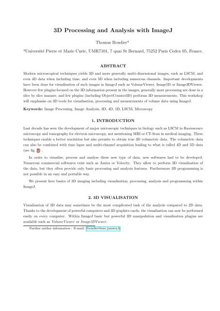
3D Processing and Analysis with ImageJ

3D Processing and Analysis with ImageJ
Thomas Boudier a
a Université Pierre et Marie Curie, UMR7101, 7 quai St Bernard, 75252 Paris Cedex 05, France.
ABSTRACT
Modern microscopical techniques yields 3D and more generally multi-dimensional images, such as LSCM, and
even 4D data when including time, and even 5D when including numerous channels. Important developments
have been done for visualisation of such images in ImageJ such as VolumeViewer, Image5D or Image3DViewer.
However few plugins focused on the 3D information present in the images, generally most processing are done in a
slice by slice manner, and few plugins (including ObjectCounter3D) performs 3D measurements. This workshop
will emphasise on 3D tools for visualisation, processing and measurements of volume data using ImageJ.
Keywords: Image Processing, Image Analysis, 3D, 4D, 5D, LSCM, Microscopy
1. INTRODUCTION
Last decade has seen the development of major microscopic techniques in biology such as LSCM in fluorescence
microscopy and tomography for electron microscopy, not mentioning MRI or CT-Scan in medical imaging. These
techniques enable a better resolution but also permits to obtain true 3D volumetric data. The volumetric data
can also be combined with time lapse and multi-channel acquisition leading to what is called 4D and 5D data
(see fig. 1) .
In order to visualise, process and analyse these new type of data, new softwares had to be developed.
Numerous commercial softwares exist such as Amira or Volocity. They allow to perform 3D visualisation of
the data, but they often provide only basic processing and analysis features. Furthermore 3D programming is
not possible in an easy and portable way.
We present here basics of 3D imaging including visualisation, processing, analysis and programming within
ImageJ.
2. 3D VISUALISATION
Visualisation of 3D data may sometimes be the most complicated task of the analysis compared to 2D data.
Thanks to the development of powerful computers and 3D graphics cards, the visualisation can now be performed
easily on every computer. Within ImageJ basic but powerful 3D manipulation and visualisation plugins are
available such as VolumeViewer or Image3DViewer.
Further author information : E-mail: tboudier@snv.jussieu.fr

Figure 1. Slice 8 from the 4D stack Organ of Corti that can be found as a sample image in ImageJ.
3D manipulation and visualisation with ImageJ
ImageJ allows the manipulation of volume data via the Stacks submenu. It allows adding or removing slices, and
animate the data. It allows also projections of the data in the Z direction, projection permits to visualise all the
3D data on one slice and increase signal to noise ratio. Volume image are represented as a succession of 2D slices
in the Z direction, the data can be resliced in X and Y direction with the Reslice command. For reslicing it is
important to take into account the spacing, i.e the size in Z of the voxel compared to its size in X − Y . Isotropic
data are usually preferred for 3D visualisation and analysis, however generally the ratio between Z spacing and
X − Y spacing is high, in order to reduce this ratio it is possible to reslice the data using the Reslice command
by specifying the input and output spacing accordingly. A volume image with additional interpolated slices will
be obtained, of course these interpolated slices do not increase the qualitative resolution in the Z direction.
In order to have an idea of the 3D presence of objects inside the volume the simplest way is to make series of
projections of the data. This will create series of projections of the data as if one was turning around the data
and view it transparent at each of these angles, thanks to a animation our brain will reconstruct the whole 3D
data. This can be done using the 3D Project command with the mean value and Y axis options.
The VolumeViewer plugin
The VolumeViewer plugin allows more complex and interactive volume visualisation. Slices in any direction can
be performed inside the volume, an orientation is chosen with the mouse and then one can scroll trough the
volume adjusting the distance view. For volume visualisation a threshold must be chosen, the voxels above this
value will be set as transparent,for other voxels the higher values the more opaque. The voxels that are visualised
are set with the depth slider.
The Image3DViewer plugin
The ImageJ3DViewer plugin requires the installation of Java3D and the presence of a 3D Graphics card. It
allows the visualisation at the same time of volume data, orthogonal slices and surfaces. In order to build

Figure 2. Two views with the Image3DViewer plugin from the red and green canal of 4D stack of Fig. 1. Left : volume
rendering, all voxels are visualised. Right : surface rendering, only thresholded voxels are seen, note that no variation of
intensities is available.
surfaces (meshes) a threshold must be chosen, a binary volume is build and voxels at the border of the binarized
objects will be displayed. Transparencies between the various representations can be adjusted allowing a complete
interactive view of multiple objects coming from the same or different volumes. Finally an animation of the 3D
visualisation can be constructed interactively and recored as a AVI movie.
HyperStacks manipulation : 4D and 5D
Volume data incorporating time or multiple channels are called HyperStacks and can be manipulated within
ImageJ. The hyperStack can be projected in Z for all channels and times, however 4D or 5D visualisation is
not (yet) possible with the 3D Project command. For 4D visualisation, that is to say animation of several 3D
dataset, the ImageJ3DViewer plugin can be used as well as other free softwares such as Voxx2.
3. 3D PROCESSING
Volmetric data may present a signal to noise ratio lower than 2D data, hence some processing may be necessary
to reduce noise and enhance signal. The theory of processing is essentially the same for 2D and 3D data, it is
based on the extraction of neighboring pixel values, the computation of the processed value from these values,
and the application of this value to the central pixel of the neighbourhood. Basically in 2D the neighbourhood
may be any symmetrical shape, usually a square or a circle. For 3D images any symmetrical shape like brick or
ellipsoid is used.
The number of values to process in 3D neighbourhood are quite larger than in 2D, for a neighbourhood
of radius 3, 9 values are present in a 2D square and 27 in a 3D cube. The time to process an image is then
considerably increased from 2D to 3D. Implementations procedure should be optimised and JNI programming
can be used. JNI programming consists in writing time-consuming procedures in other languages like C, that is
quite faster than Java.

Figure 3. “ THe stack of Fig. 1 was denoised by a 3D median filter of radius 1. Left : volume rendering. Right : surface
rendering, note that surfaces are smoother.
In this section we describe commonly used filtering and morphological operators, but first a introduction to
contrast adjustment.
Brightness and contrast
Brightness and contrast may be adjusted slice by slice to improve the visualisation of objects of interest. However
changes in contrast may be present from slice to slice due to the acquisition procedure, like decrease of fluorescence
for LSCM or increase of thickness in tilted series for electron tomography. These changes in contrast can be
modelled and the contrast can be corrected based on the model. The contrast can be also automatically adjusted
from slice to slice thanks to the Normalise All slice command of the Enhance Contrast function. This procedure
will process the data so that the the slices will have roughly the same mean and standard deviation, correcting
hence any changes in contrast trough the data.
Noise reduction
Volume data can be 2D-filtered in a slice by slice manner, this can produce fast satisfactory results but in some
cases, where the signal to noise ratio is quite low, a 3D filtering should be favoured. Very weak signals are present
in 3D, that is to say on adjacent slices, they may however be almost indistinguishable in 2D due to noise. Only
a 3D filtering can take into account the 3D information of the signal and reduce the noise. Classical filters used
for reducing noise are mean, gaussian or median filters. Median filter can be favoured since it is more robust to
noise and preserve the edges of the objects, it is specially powerful on noisy confocal data images.
The radius of filtering should be chosen accordingly to the size of the objects of interest since filtering reduces
noise but also may suppress small objects, the smaller the objects the lower the radius. The choice of the radius
obeys the same rule in 2D as in 3D. However due to the acquisition systems, objects tend to be a bit elongated
in Z compared to X − Y , furthermore the spacing is generally different in Z than in X − Y so round objects do
not have the same radius in pixels in Z than in X − Y , the radius of filtering should hence be different in the
two directions. The radii of the neighborhood kernel can also be optimally computed for each voxel in order to

fit inside a probable object and avoiding averaging between signals and background. Such procedures are part
of anisotropic filtering,
Morphology
Mathematical morphology is originally based on complex mathematical operations between sets, however applied
to images it can be seen as a particular type of filtering. Morphological operations are to be applied to binarized
images and work on the objects segmented by the binarization. However many operations can be extended to
grey-level images. The basic operation of mathematical morphology is called dilatation and consist in superim-
posing a kernel to every pixel of the image, and if any of the pixel in the kernel is part of an object then the
centre of the kernel turns to the objects value. Contrary to filtering the kernel does not need to be symmetrical,
however usually a symmetrical kernel is used. The inverse operation of dilatation is called erosion, the centre of
the kernel turns to the background value if any of the pixel inside the kernel is part of the background. For 3D
morphology the kernel is a 3D shape, usually a ellipsoid or a 3D brick.
Actually useful moprhological operations are a combination of the two basics operation, for instance closing
consists in a dilatation followed by an erosion and permits to make the objects more compact and fills small holes
inside objects. The twin operation opening, a erosion followed by a dilatation, permits to remove small spots in
the background. Other useful operations are fill holes to suppress any hole present within an object, distance
map to compute for any pixel its distance to the closest edge or tophat to enhance spots. This operation consists
in computing a local background image by removing the objects, and then to perform the difference between
the original image and the computed background. In the case of bright spots the background is computed by
performing a minimum filter, equivalent to an erosion, hence removing any bright signal. The size of the kernel
must therefore be larger that the object size. This procedure is quite powerful in 3D to detect fluorescence signals
like F.I.S.H. spots.
Other processing
Any procedure that processes a 2D image via a kernel can be quite directly adapted to 3D data, however the
main concern is time and memory requirements since a 3D image can be hundred times bigger than a 2D image.
Another purpose of filtering is edge detection, in 2D a classical way to detect edges is to compute edges in
both X and Y directions and then combine them to find the norm of the gradient corresponding to the strength
of the edges, the angle of the edges can also be computed from the X and Y differentials. For 3D edges the
differential in Z is added to the X and Y ones.
δx(i, j, k) ≈ I(i + 1, j, k) − I(i − 1, j, k),
δy(i, j, k) ≈ I(i, j + 1, k) − I(i, j − 1, j),
δz(i, j, k) ≈ I(i, j, k + 1) − I(i, j, k − 1),
edge = δx 2 + δy 2 + δz 2
Fourier processing
The above cited processing were performed on the real images, other processing can be performed on the Fourier
transform of the image. The Fourier transform of the image corresponds to the frequencies inside the real image,
so, in another way, to the various sizes of objects present in the image. In order to reduce noise objects with very
small sizes, hence high frequencies, can be deleted using a low pass filter. To enhance objects with a particular

size band pass filtering can be performed, see the Bandpass Filter in the FFT menu. The Fourier Transform
can also be computed in 3D, however the computation time can be quite long if non power of 2 images are used.
Other applications of Fourier Transform are signal deconvolution and correlation computations, that permits to
find the best displacement in X, Y and Z between two volumes.
For stack alignment the computation of the 3D translation between two volumes can be easily computed
in Fourier Space, however for computation of 3D rotation the problem is quite more complex than in 2D since
3 angles, around each axis, must be computed. Complex optimisation algorithm should be used, iterative
procedures including translation and rotations estimations are generally used, see the StackAlignment plugin.
4. 3D SEGMENTATION
Segmentation is the central procedure in image analysis. It permits to give a meaning to an image by extracting
the objects, that are actually no more than a set of numeric values. The labelling of pixels to a numbered object
or to background is the most difficult task of image analysis since we have to teach the computer what are
objects, for instance what is a cell, what is a nucleus, what is an axon and so on.
The task is quite more complicated in 3D since it is more difficult to describe a 3D shape than a 2D one. To
perform the labelling of objects, two main approaches can be used; first objects can either be drawn manually
either extracted based on their voxels values. Active contours model, known as snakes, is a semi-automatic
approach where the user draw a rough initial shape and the computer will try to deform this shape to best fit
the surrounding contour.
Thresholding
If the objects have homogeneous pixel values and if the values are significatively different from the background, a
thresholding can be applied. In the case of an inhomogeneous illumination of the image the Substract Background
procedure should be used. The Adjust Threshold tool helps in determining the threshold, an interval of values is
manually selected and the thresholded pixels, corresponding to the objects, are displayed in red colour. Automatic
threshold can be computed using various algorithms like IsoData, Maximum of Entropy, Otsu,
Thresholding in 3D obeys the same rules, however the object may present intensity variation in the Z
direction. This variation can be corrected by a normalisation procedure (see 3). An automatic calculation of the
threshold can also be computed in each individual slices, but due to normal variation of objects intensities in Z
this procedure is not well adapted for 3D segmentation.
After thresholding, objects should be labelled, that is to say numbered. The Analyse Particles procedure
perform this task in 2D, it can be applied to 3D but it will label objects in each slices not taking into account
the third dimension. Furthermore objects that look separated in 2D may be part of the same object in 3D,
for instance a simple banana shape may present its two ends separated in a 2D section. Hence a true 3D
labelling should be performed, the plugin ObjectCounter3D will both threshold and label the objects in 3D. It
also computes geometrical measures like volume and surfaces.
Manual segmentation
In some cases the objects can not be thresholded in a satisfying way. Morphology procedures (see 3) may
improve the binarization result, but for some complex objects, as ones observed by electron microscopy, a
manual segmentation is required. The user have to draw in each slices the contours of the different objects.

Figure 4. Output of the sample data from fig. 1 with the ObjectCounter3D plugin, objects are segmented in 3D and
labelled with an unique index, displayed here with a look-up table. Left : red channel, note that some objects are fused.
Right : green channels, note all that fibers form only one object.
Some plugins can help the user in this task such as QuickvolII mainly for MRI, TrackEM2 (see Workshop on this
subject) or SegmentationEditor, other free tools exist like IMOD mainly specialised in electron microscopy data.
Semi-automatic segmentation : active contours
Active contours models, known as snakes, are semi automatic techniques that can help the user automate a
manual segmentation. The user draws the initial model close to the object he wants to segment, the algorithm
will then try to deform this initial shape so that it fits onto the contours of the image. Many algorithms are
available as plugins such as IVUSnake, Snakuscule, or ABSnake.
Snakes model, though developed for 2D data, can be used in 3D in a iterative manner. The user draws an
initial shape on the first slice of the volume, the algorithm will then segment the object, this segmentation on
the first slice can be used as the initial shape for the next slice, and so on. However this method does not take
into account the 3D information and the links that exist between adjacent slices. Furthermore in the case of
noisy data or problem in acquisition an object can be missing or deformed in a particular slice. The slice by slice
approach can not alleviate this problem, a real 3D procedure that take into account data in adjacent slices, as
it is done in X − Y should be used. The plugin ABSnake3D uses such an approach, the model is a set of points
lying in the different slices. For each iteration the point will move towards the contours of the image while being
constrained in X − Y by its two neighboring points and also in Z by the two closest points in the upper and
lower slices.
5. 3D ANALYSIS
Once the objects have been segmented the analysis can be performed. This part will compute geometrical and
pixel-based measures for each individual object. These measures must be performed using the real units of the
image. The image should hence be calibrated in the 3 dimensions thanks to the Image/Properties window.

Figure 5. The 3DManager plugin in action. Objects are added to the manager via the segmented image of fig. 4. The
objects 6 and 10 were selected and measured. Geometrical measures appear in the 3D Measure results window, the canal
1 window was selected and intensity measures from this image appear in the 3D quantif results window.
Geometrical features
The geometrical features concern the shape of the object without taking into account its intensitiy values. Basic
measures are volume and area. Volume is actually the number of voxels belonging to the object and can be
computed as the sum of 2D areas multiplied by the Z spacing. The area of a 3D object corresponds to the
number of voxels at its border, however the border can be defined in several ways, for instance allowing diagonal
voxels or not, and hence the computation of area may vary from a program to another. From this basic measures
one can compute the 3D sphericity which is an extension of 2D circularity, and is computed from the ratio of
volume over area. The sphericity, as well as the circularity, is maximal and equals 1 for a sphere : S 3 =
with S being the sphericity, V the volume and A the area.
2
36.Π.V
A3 ,
Other measures like Feret diameter or ellipsoid fitting can not be computed from 2D slices, contrary to volume
or area. Feret diameter is the longest distance from two contour points of the 3D object. In order to have an
idea of the global orientation of the object the fitting a 3D ellipsoid can be used. Actually the main axes of the
3D shape can be computed as the eigen vectors of the following moments matrix :
with :
⎛
⎞
sxx sxy sxz
⎜
⎟
⎝syx
syy syz⎠
szx szy szz

Figure 6. Distance computation with the 3DManager plugin. The objects from red and green channels were added to
the manager. The distances between objects 6 and 10 from red canal and object 1 (representing the fibers) from green
canal were computed. From border to border distances one can see that object 10 touches the fibers.
sxx = (x − cx).(x − cx),
syy = (y − cy).(y − cy),
szz = (z − cz).(z − cz),
sxy = syx = (x − cx).(y − cy),
sxz = szx = (x − cx).(z − cz),
syz = szy = (y − cy).(z − cz),
x, y and z being the coordinates of the points belonging to the object, cx, cy, cz being the coordinates of the
barycentre of the object. The 3 eigen vectors will correspond to the 3 main axes of the shape. An elongation
factor can be computed as the ratio between the two eigen values of the two first main axes.
Other geometrical measures can give valuable information like distances between objects. The distances can
be computed from centre to centre, or from border to border giving the minimal distance between objects. One
may also be interested by the distance from the centre of an object to the border of another, or the distance
along a particular direction. One may also be interested in the percentage of inclusion of an object into another,
and so on.
Finally the shape of the envelope of the object can be studied, in 2D this envelope correspond to the perimeter
of the object and can be mathematically analysed as a curve, hence information like curvature can be computed.
In 3D such analysis is quite more complex since the border corresponds to a mathematical surface, and for
instance for each point of a surface there are two curvatures instead of one.
Intensity features
The above geometrical measures do not not take into account the intensity of the voxels inside the object. In
the case of an inhomogeneous distribution of the gray-levels inside the objects, intensity-based measure may
be needed. For instance Integrated Density, which is the volume multiplied by the mean voxel value inside the
object, and correspond to the sum of intensities inside the object. Mass centres are the barycenter of the voxels

Ip.x
weighted by the pixel intensities : MCx = , where Ip is the intensity at point p belonging to the object
Ip
and x its x-coordinate, same applies for y and z.
Main axes can also be computed by weighting all coordinates by the voxel value. Note that in most cases, due
to the segmentation process, the object present homogeneous intensities and hence intensity-based barycenter
and axes does not differ much from those computed in the above paragraph where actually all voxels are weighted
by a factor of 1.
Morphological analysis
A first application of mathematical morphology is the computation of 3D local thickness based on the distance
map. For each point inside the object its minimum distance to the border can be used as an estimate to the
maximal sphere that can be fitted at this point inside the object.
Mathematical morphology can be used to fill holes inside objects or make them more compact, it can also
be used to have a estimate of the sizes of the objects present in the volume without to segment them. The
technique, called granulometry, is based on the idea that objects processed by an erosion greater than the radius
of the object will disappear. For grey-levels volumes, an erosion is actually a minimum filter, hence if bright
objects are present in the image, and if the radius of the minimum filter is greater than the radius of the object,
the minimum value inside the neighbourhood will be in the background. This will occur for any pixel inside the
object and hence the object will tend to disappear. Therefore computing series of opening, an erosion followed
by a dilatation, will produce series of filtered images, and the image that will differ much from the original
will correspond to the disappearing of many objects, the corresponding radius of opening will correspond to the
radius of some objects present in the volume. If many objects are present with different radii, for each particular
radius the image will change. The same can be done with series of closing, dilatation followed by an erosion, in
this case, radius of background will be detected, that is to say distances between objects.
6. 3D PROGRAMMING
Many, if not all, operations implemented in ImageJ can be performed on 3D data on a slice by slice manner.
Hence macro recording should be sufficient to record series of processing performed on a stack by either ImageJ
or plugins. For 3D analysis access to all the slices is often required. This can be done in macros using the slices
commands, and the ImageStack class in plugins.
Macros
In order to manipulate a stack, the different slices corresponding to different z should be accessed. This can be
done using the macro command setSlice(n) where n is the slice number between 1 and the total number of
slices. The current displayed slice can be retrieved using the command getSliceNumber(), nSlices is a built-in
variable corresponding to the total number of slices. In order to scroll trough the slices a loop is required, a loop
is constructed by the for command : for(index=start;index

areamax=0;
slicemax=start;
run("Set Measurements...", "area redirect=None decimal=3");
for(slice=start;sliceareamax){
}
areamax=area;
slicemax=slice;
write("Max area at slice "+slicemax);
getVoxelSize(sizex,sizey,sizez,unit);
write("Max area at z "+slicemax*sizez+" "+unit);
For 4D and 5D data, the macro functions Stack. should be used. The various dimensions, that is to say the
width, height, number of channels, number of slices and number of times, can be retrieved using the function
Stack.getDimensions(width,height,channels,slices,frames). The equivalent of setSlice(n) is simply
Stack.setSlice(n) for HyperStacks, similarly the functions Stack.setChannel(n) and Stack.setFrame(n)
will change the channel and timepoint. The different information can be set using one function
Stack.setPosition(channel,slice,frame) and retrieved by the function
Stack.getPosition(channel,slice,frame). The same macro is rewritten supposing a 4D data :
Stack.getPosition(channel,slice,frame);
startTime=frame;
startZ=slice;
Stack.getDimensions(w,h,channels,slices,frames);
endTime=frames;
endZ=slices;
run("Set Measurements...", "area redirect=None decimal=3");
getVoxelSize(sizex,sizey,sizez,unit);
for(time=startTime;time

}
Plugins
}
}
areamax=area;
slicemax=slice;
write("For time "+time+" Max area at slice "+slicemax);
write("For time "+time+" Max area at z "+slicemax*sizez+" "+unit);
Plugins are more adapted than macros to implement new processing procedures since the pixels access is quite
faster. The Java class that stores stacks is called ImageStack, the stack can be retrieved from the current
ImagePlus window :
// get current image and get its stack
ImagePlus plus=IJ.getImage();
ImageStack stack=plus.getStack();
The dimensions of the stack can be obtained using the methods getWidth(), getHeight() and getSize():
int w=stack.getWidth();
int h=stack.getHeight();
int d=stack.getSize();
IJ.write("dimensions : "+w+" "+h+" "+d);
slice :
In order to access the pixels values one has to access first the slice of interest and then the pixel inside this
int x,y,z;
x=w/2; y=h/2; z=d/2;
ImageProcessor slice=stack.getProcessor(z+1);
int val=slice.getPixel(x,y);
IJ.write("The central pixel has value : "+val);
Note that the slice number in the getProcessor method starts at 1 and not 0. Following is an example of a 3D
mean filtering :
int p0,p1,p2,p3,p4,p5,p6,mean;
ImageStack filtered=new ImageStack(w,h);
ImageProcessor filteredSlice;
ImageProcessor slice, sliceUp, sliceDown;
for(int k=2;k

}
filteredSlice=new ByteProcessor(w,h);
for(int i=1;i

stack is a stack containing segmented objects, each one having a particular grey-level
// for instance coming from ObjectCounter3D
IntImage3D seg = new IntImage3D(stack);
// create the object 1, which corresponds to segmented voxels having values 1
obj = new Object3D(seg, 1);
// compute barycenter
obj.computeCenter();
// compute borders
obj.computeContours();
// get barycenter
float bx = obj.getCenterX();
float by = obj.getCenterY();
float bz = obj.getCenterZ();
// get the feret’s diameter
double feret = obj.getFeret();
// construct an sphere with pixel value 255 centered on barycenter and with radius=feret
ObjectCreator3D sphere = new ObjectCreator3D(w, h, d);
obj.createEllipsoide(bx, by, bz, feret, feret, feret, 255);
new ImagePlus("Sphere", sphere.getStack()).show();
APPENDIX A. LIST OF PLUGINS
• VolumeViewer : http://rsbweb.nih.gov/ij/plugins/volume-viewer.html
• ImageJ3DViewer and 3D Segmentation Editor : http://www.neurofly.de/
• Image5D : http://rsbweb.nih.gov/ij/plugins/image5d.html
• IJ3D processing and analysis : http://imagejdocu.tudor.lu/doku.php
• StackAlignment : http://www.med.harvard.edu/JPNM/ij/plugins/Align3TP.html
• ObjectCounter3D : http://rsbweb.nih.gov/ij/plugins/track/objects.html
• ABSnake : http://imagejdocu.tudor.lu/doku.php?id=plugin:segmentation:active_contour:start
• LiveWire and IVUSnake : http://ivussnakes.sourceforge.net/
• Snakuscule : http://bigwww.epfl.ch/thevenaz/snakuscule/
• TrackEM2 : http://www.ini.uzh.ch/~acardona/trakem2.html
• QuickVol II : http://www.quickvol.com/

APPENDIX B. OTHER PROGRAMS
• IMOD 3D segmentation and visualisation : http://bio3d.colorado.edu/imod/
• Voxx2 3D and 4D visualisation : http://www.nephrology.iupui.edu/imaging/voxx/
• 3D molecular visualisation : http://www.cgl.ucsf.edu/chimera/
• Etdips 3D medical analysis and visualisation : http://www.cc.nih.gov/cip/software/etdips/
ACKNOWLEDGMENTS
I would like to thanks all 3D developers for ImageJ. Special thank to C. Messaoudi who developed the first
version of the ij3d library and P. Andrey for fruitful discussion and the implementation of the 3D version of
ABSnake.