ifrender - Nanyang Technological University

6 • Wu et al.
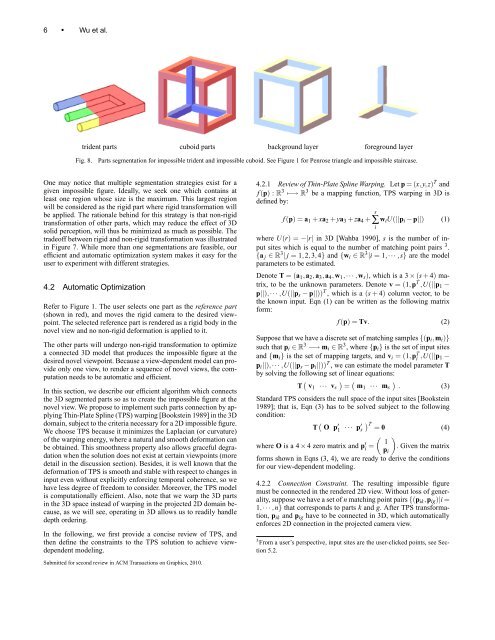
trident parts cuboid parts background layer foreground layer
Fig. 8. Parts segmentation for impossible trident and impossible cuboid. See Figure 1 for Penrose triangle and impossible staircase.
One may notice that multiple segmentation strategies exist for a
given impossible figure. Ideally, we seek one which contains at
least one region whose size is the maximum. This largest region
will be considered as the rigid part where rigid transformation will
be applied. The rationale behind for this strategy is that non-rigid
transformation of other parts, which may reduce the effect of 3D
solid perception, will thus be minimized as much as possible. The
tradeoff between rigid and non-rigid transformation was illustrated
in Figure 7. While more than one segmentations are feasible, our
efficient and automatic optimization system makes it easy for the
user to experiment with different strategies.
4.2 Automatic Optimization
Refer to Figure 1. The user selects one part as the reference part
(shown in red), and moves the rigid camera to the desired viewpoint.
The selected reference part is rendered as a rigid body in the
novel view and no non-rigid deformation is applied to it.
The other parts will undergo non-rigid transformation to optimize
a connected 3D model that produces the impossible figure at the
desired novel viewpoint. Because a view-dependent model can provide
only one view, to render a sequence of novel views, the computation
needs to be automatic and efficient.
In this section, we describe our efficient algorithm which connects
the 3D segmented parts so as to create the impossible figure at the
novel view. We propose to implement such parts connection by applying
Thin-Plate Spline (TPS) warping [Bookstein 1989] in the 3D
domain, subject to the criteria necessary for a 2D impossible figure.
We choose TPS because it minimizes the Laplacian (or curvature)
of the warping energy, where a natural and smooth deformation can
be obtained. This smoothness property also allows graceful degradation
when the solution does not exist at certain viewpoints (more
detail in the discussion section). Besides, it is well known that the
deformation of TPS is smooth and stable with respect to changes in
input even without explicitly enforcing temporal coherence, so we
have less degree of freedom to consider. Moreover, the TPS model
is computationally efficient. Also, note that we warp the 3D parts
in the 3D space instead of warping in the projected 2D domain because,
as we will see, operating in 3D allows us to readily handle
depth ordering.
In the following, we first provide a concise review of TPS, and
then define the constraints to the TPS solution to achieve viewdependent
modeling.
Submitted for second review in ACM Transactions on Graphics, 2010.
4.2.1 Review of Thin-Plate Spline Warping. Let p = (x,y,z) T and
f(p) : R 3 ↦−→ R 3 be a mapping function, TPS warping in 3D is
defined by:
s
f(p) = a1 + xa2 + ya3 + za4 + ∑wiU(||pi − p||) (1)
i
where U(r) = −|r| in 3D [Wahba 1990], s is the number of input
sites which is equal to the number of matching point pairs 3 .
{a j ∈ R 3 | j = 1,2,3,4} and {wi ∈ R 3 |i = 1,··· ,s} are the model
parameters to be estimated.
Denote T = (a1,a2,a3,a4,w1,··· ,ws), which is a 3 ×(s+4) matrix,
to be the unknown parameters. Denote v = (1,p T ,U(||p1 −
p||),··· ,U(||ps − p||)) T , which is a (s + 4) column vector, to be
the known input. Eqn (1) can be written as the following matrix
form:
f(p) = Tv. (2)
Suppose that we have a discrete set of matching samples {(pi,mi)}
such that pi ∈ R3 −→ mi ∈ R3 , where {pi} is the set of input sites
and {mi} is the set of mapping targets, and vi = (1,pT i ,U(||p1 −
pi||),··· ,U(||ps − pi||)) T , we can estimate the model parameter T
by solving the following set of linear equations:
T
v1 ··· vs = m1 ··· ms . (3)
Standard TPS considers the null space of the input sites [Bookstein
1989]; that is, Eqn (3) has to be solved subject to the following
condition:
T O p ′ 1 ··· p′ T s = 0
(4)
. Given the matrix
where O is a 4 × 4 zero matrix and p ′ i =
1
pi
forms shown in Eqns (3, 4), we are ready to derive the conditions
for our view-dependent modeling.
4.2.2 Connection Constraint. The resulting impossible figure
must be connected in the rendered 2D view. Without loss of generality,
suppose we have a set of n matching point pairs {(pik,pig)|i =
1,··· ,n} that corresponds to parts k and g. After TPS transformation,
pik and pig have to be connected in 3D, which automatically
enforces 2D connection in the projected camera view.
3 From a user’s perspective, input sites are the user-clicked points, see Sec-
tion 5.2.