Chapter 5 - WebRing

CHAPTER 5. MAGNETIC SYSTEMS 261
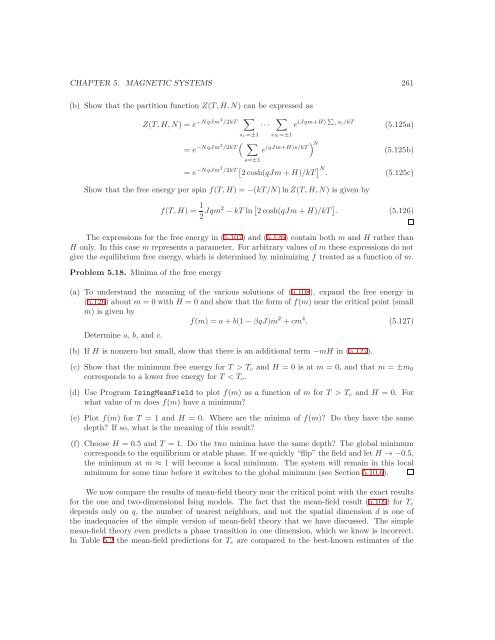
(b) Show that the partition function Z(T,H,N) can be expressed as
Z(T,H,N) = e −NqJm2 /2kT
···
e (Jqm+H) i si/kT
s1=±1
= e −NqJm2 /2kT
s=±1
sN=±1
e (qJm+H)s/kT N
(5.125a)
(5.125b)
= e −NqJm2 /2kT 2cosh(qJm+H)/kT N . (5.125c)
Show that the free energy per spin f(T,H) = −(kT/N)lnZ(T,H,N) is given by
f(T,H) = 1
2 Jqm2 −kT ln 2cosh(qJm+H)/kT . (5.126)
The expressions for the free energy in (5.107) and (5.126) contain both m and H rather than
H only. In this case m represents a parameter. For arbitrary values of m these expressions do not
give the equilibrium free energy, which is determined by minimizing f treated as a function of m.
Problem 5.18. Minima of the free energy
(a) To understand the meaning of the various solutions of (5.108), expand the free energy in
(5.126) about m = 0 with H = 0 and show that the form of f(m) near the critical point (small
m) is given by
f(m) = a+b(1−βqJ)m 2 +cm 4 . (5.127)
Determine a, b, and c.
(b) If H is nonzero but small, show that there is an additional term −mH in (5.127).
(c) Show that the minimum free energy for T > Tc and H = 0 is at m = 0, and that m = ±m0
corresponds to a lower free energy for T < Tc.
(d) Use Program IsingMeanField to plot f(m) as a function of m for T > Tc and H = 0. For
what value of m does f(m) have a minimum?
(e) Plot f(m) for T = 1 and H = 0. Where are the minima of f(m)? Do they have the same
depth? If so, what is the meaning of this result?
(f) Choose H = 0.5 and T = 1. Do the two minima have the same depth? The global minimum
correspondsto the equilibrium or stable phase. If we quickly “flip” the field and let H → −0.5,
the minimum at m ≈ 1 will become a local minimum. The system will remain in this local
minimum for some time before it switches to the global minimum (see Section 5.10.6).
We now compare the results of mean-field theory near the critical point with the exact results
for the one and two-dimensional Ising models. The fact that the mean-field result (5.109) for Tc
depends only on q, the number of nearest neighbors, and not the spatial dimension d is one of
the inadequacies of the simple version of mean-field theory that we have discussed. The simple
mean-field theory even predicts a phase transition in one dimension, which we know is incorrect.
In Table 5.2 the mean-field predictions for Tc are compared to the best-known estimates of the