Chapter 5 - WebRing
Chapter 5 - WebRing
Chapter 5 - WebRing

You also want an ePaper? Increase the reach of your titles
YUMPU automatically turns print PDFs into web optimized ePapers that Google loves.
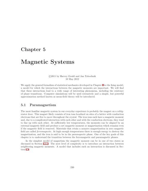
<strong>Chapter</strong> 5<br />
Magnetic Systems<br />
c○2011 by Harvey Gould and Jan Tobochnik<br />
10 May 2012<br />
We apply the general formalism of statistical mechanics developed in <strong>Chapter</strong> 4 to the Ising model,<br />
a model for which the interactions between the magnetic moments are important. We will find<br />
that these interactions lead to a wide range of interesting phenomena, including the existence<br />
of phase transitions. Computer simulations will be used extensively and a simple, but powerful<br />
approximation method known as mean-field theory will be introduced.<br />
5.1 Paramagnetism<br />
The most familiar magnetic system in our everyday experience is probably the magnet on a refrigerator<br />
door. This magnet likely consists of iron ions localized on sites of a lattice with conduction<br />
electrons that are free to move throughout the crystal. The iron ions each have a magnetic moment<br />
and, due to a complicated interaction with each other and with the conduction electrons, they tend<br />
to line up with each other. At sufficiently low temperatures, the moments can be aligned by an<br />
external magnetic field and produce a net magnetic moment or magnetization which remains even<br />
if the magnetic field is removed. Materials that retain a nonzero magnetization in zero magnetic<br />
field are called ferromagnetic. At high enough temperatures there is enough energy to destroy the<br />
magnetization, and the iron is said to be in the paramagnetic phase. One of the key goals of this<br />
chapter is to understand the transition between the ferromagnetic and paramagnetic phases.<br />
In the simplest model of magnetism the magnetic moment can be in one of two states as<br />
discussed in Section 4.3.1. The next level of complexity is to introduce an interaction between<br />
neighboring magnetic moments. A model that includes such an interaction is discussed in Section<br />
5.4.<br />
230
CHAPTER 5. MAGNETIC SYSTEMS 231<br />
5.2 Noninteracting Magnetic Moments<br />
We first review the behavior of a system of noninteracting magnetic moments with spin 1/2 in<br />
equilibrium with a heat bath at temperature T. We discussed this system in Section 4.3.1 and in<br />
Example 4.1 using the microcanonical ensemble.<br />
The energy of interaction of a magnetic moment µ in a magnetic field B is given by<br />
E = −µ·B = −µzB, (5.1)<br />
where µz is the component of the magnetic moment in the direction of the magnetic field B.<br />
Because the magnetic moment has spin 1/2, it has two possible orientations. We write µz = sµ,<br />
where s = ±1. The association of the magnetic moment of a particle with its spin is an intrinsic<br />
quantum mechanical effect (see Section 5.10.1). We will refer to the magnetic moment or the spin<br />
of a particle interchangeably.<br />
What would we like to know about the properties of a system of noninteracting spins? In the<br />
absence of an external magnetic field, there is little of interest. The spins point randomly up or<br />
down because there is no preferred direction, and the mean internal energy is zero. In contrast, in<br />
the presence of an external magnetic field, the net magnetic moment and the energy of the system<br />
are nonzero. In the following we will calculate their mean values as a function of the external<br />
magnetic field B and the temperature T.<br />
We assume that the spins are fixed on a lattice so that they are distinguishable even though<br />
the spins are intrinsically quantum mechanical. Hence the only quantum mechanical property of<br />
the system is that the spins are restricted to two values. As we will learn, the usual choice for<br />
determining the thermal properties of systems defined on a lattice is the canonical ensemble.<br />
Because each spin is independent of the others and distinguishable, we can find the partition<br />
function for one spin, Z1, and use the relation ZN = ZN 1 to obtain ZN, the partition function for<br />
N spins. (We reached a similar conclusion in Example 4.2.) We can derive this relation between<br />
Z1 and ZN by writing the energy of the N spins as E = −µB N i=1si and expressing the partition<br />
function ZN for the N-spin system as<br />
To find Z1 we write<br />
ZN = <br />
<br />
s1=±1 s2=±1<br />
= <br />
<br />
s1=±1 s2=±1<br />
= <br />
s1=±1<br />
e βµBs1<br />
<br />
= e βµBs1<br />
Z1 = <br />
s=±1<br />
s1=±1<br />
... <br />
sN=±1<br />
... <br />
sN=±1<br />
<br />
s2=±1<br />
N = Z N 1<br />
e βµBΣN<br />
i=1 si (5.2a)<br />
e βµBs1 e βµBs2 ...e βµBsN (5.2b)<br />
e βµBs2 ... <br />
sN=±1<br />
e βµBsN (5.2c)<br />
. (5.2d)<br />
e βµBs = e βµB(−1) +e βµB(+1) = 2coshβµB. (5.3)
CHAPTER 5. MAGNETIC SYSTEMS 232<br />
Hence, the partition function for N spins is<br />
ZN = (2coshβµB) N . (5.4)<br />
We now use the canonical ensemble formalism that we developed in Section 4.6 to find the<br />
thermodynamic properties of the system for a given T and B. The free energy is given by<br />
The mean energy E is<br />
F = −kT lnZN = −NkT lnZ1 = −NkT ln(2coshβµB). (5.5)<br />
E = − ∂lnZN<br />
∂β<br />
= ∂(βF)<br />
∂β<br />
= −NµB tanhβµB. (5.6)<br />
From (5.6) we see that E → 0 as T → ∞ (β → 0). In the following we will frequently omit the<br />
mean value notation when it is clear from the context that an average is implied.<br />
Problem 5.1. Comparison of the results for two ensembles<br />
(a) Compare the result (5.6) for the mean energy E(T) of a system of noninteracting spins in<br />
the canonical ensemble to the result that you found in Problem 4.21 for T(E) using the<br />
microcanonical ensemble.<br />
(b) Why is it much easier to treat a system of noninteracting spins in the canonical ensemble?<br />
(c) What is the probability p that a spin is parallel to the magnetic field B given that the system<br />
is in equilibrium with a heat bath at temperature T? Compare your result to the result in<br />
(4.74) using the microcanonical ensemble.<br />
(d) What is the relation of the results that we have found for a system of noninteracting spins to<br />
the results obtained in Example 4.2?<br />
The heat capacity C is a measure of the change of the temperature due to the addition of<br />
energy at constant magnetic field. The heat capacity at constant magnetic field can be expressed<br />
as<br />
C =<br />
<br />
∂E<br />
<br />
∂T B<br />
= −kβ2∂E . (5.7)<br />
∂β<br />
(We will write C rather than CB.) From (5.6) and (5.7) we find that the heat capacity of a system<br />
of N noninteracting spins is given by<br />
C = kN(βµB) 2 sech 2 βµB. (5.8)<br />
Note that the heat capacity is always positive, goes to zero at high T, and goes to zero as T → 0,<br />
consistent with the third law of thermodynamics.<br />
Magnetization and susceptibility. Two other macroscopic quantities of interest for magnetic<br />
systems are the mean magnetization M (in the z direction) given by<br />
M = µ<br />
N<br />
si, (5.9)<br />
i=1
CHAPTER 5. MAGNETIC SYSTEMS 233<br />
and the isothermal susceptibility χ, which is defined as<br />
<br />
∂M<br />
<br />
χ = . (5.10)<br />
∂B T<br />
The susceptibility χ is a measure of the change of the magnetization due to the change in the<br />
external magnetic field and is another example of a response function.<br />
We will frequently omit the factor of µ in (5.9) so that M becomes the number of spins<br />
pointing in a given direction minus the number pointing in the opposite direction. Often it is more<br />
convenient to workwith the mean magnetization per spin m, an intensive variable, which is defined<br />
as<br />
m = 1<br />
M. (5.11)<br />
N<br />
As for the discussion of the heat capacity and the specific heat, the meaning of M and m will be<br />
clear from the context.<br />
We can express M and χ in terms of derivatives of lnZ by noting that the total energy can<br />
be expressed as<br />
E = E0 −MB, (5.12)<br />
where E0 is the energy of interaction of the spins with each other (the energy of the system when<br />
B = 0) and −MB is the energy of interaction of the spins with the external magnetic field. (For<br />
noninteracting spins E0 = 0.) The form of E in (5.12) implies that we can write Z in the form<br />
Z = <br />
e −β(E0,s−MsB) , (5.13)<br />
where Ms and E0,s are the values of M and E0 in microstate s. From (5.13) we have<br />
∂Z<br />
∂B<br />
and hence the mean magnetization is given by<br />
M = 1 <br />
Mse<br />
Z<br />
−β(E0,s−MsB)<br />
s<br />
<br />
= βMse −β(E0,s−MsB) , (5.14)<br />
s<br />
= 1<br />
βZ<br />
s<br />
∂Z<br />
∂B<br />
If we substitute the relation F = −kT lnZ, we obtain<br />
(5.15a)<br />
∂lnZN<br />
= kT . (5.15b)<br />
∂B<br />
M = − ∂F<br />
. (5.16)<br />
∂B<br />
Problem 5.2. Relation of the susceptibility to the magnetization fluctuations<br />
Use considerations similar to that used to derive (5.15b) to show that the isothermal susceptibility<br />
can be written as<br />
χ = 1<br />
kT [M2 −M 2 ] . (5.17)<br />
Note the similarity of the form (5.17) with the form (4.88) for the heat capacity CV.
CHAPTER 5. MAGNETIC SYSTEMS 234<br />
The relation of the response functions CV and χ to the equilibrium fluctuations of the energy<br />
and magnetization, respectively, are special cases of a general result known as the fluctuationdissipation<br />
theorem.<br />
Example 5.1. Magnetization and susceptibility of a noninteracting system of spins<br />
From (5.5) and (5.16) we find that the mean magnetization of a system of noninteracting spins is<br />
M = Nµ tanh(βµB). (5.18)<br />
The susceptibility can be calculated using (5.10) and (5.18) and is given by<br />
χ = Nµ 2 β sech 2 (βµB). (5.19)<br />
♦<br />
Note that theargumentsofthe hyperbolicfunctions in (5.18)and (5.19) mustbe dimensionless<br />
and be proportional to the ratio µB/kT. Because there are only two energy scales in the system,<br />
µB, the energyofinteractionof aspin with the magneticfield, and kT, the argumentsmust depend<br />
only on the dimensionless ratio µB/kT.<br />
For high temperatures kT ≫ µB (βµB ≪ 1), sech(βµB) → 1, and the leading behavior of χ<br />
is given by<br />
χ → Nµ 2 β = Nµ2<br />
(kT ≫ µB). (5.20)<br />
kT<br />
The result (5.20) is known as the Curie form of the isothermal susceptibility and is commonly<br />
observed for magnetic materials at high temperatures.<br />
From (5.18) we see that M is zero at B = 0 for all T > 0, which implies that the system is<br />
paramagnetic. Because a system of noninteracting spins is paramagnetic, such a model is not applicable<br />
to materials such as iron which can have a nonzero magnetization even when the magnetic<br />
field is zero. Ferromagnetism is due to the interactions between the spins.<br />
Problem 5.3. Thermodynamics of noninteracting spins<br />
(a) Plot the magnetization given by (5.18) and the heat capacity C given in (5.8) as a function of<br />
T for a given external magnetic field B. Give a simple argument why C must have a broad<br />
maximum somewhere between T = 0 and T = ∞.<br />
(b) Plot the isothermal susceptibility χ versus T for fixed B and describe its limiting behavior for<br />
low temperatures.<br />
(c) Calculate the entropy of a system of N noninteracting spins and discuss its limiting behavior<br />
at low (kT ≪ µB) and high temperatures (kT ≫ µB). Does S depend on kT and µB<br />
separately?<br />
Problem 5.4. Adiabatic demagnetization<br />
Consider a solid containing N noninteracting paramagnetic atoms whose magnetic moments can<br />
be aligned either parallel or antiparallel to the magnetic field B. The system is in equilibrium with<br />
a heat bath at temperature T. The magnetic moment is µ = 9.274×10 −24 J/tesla.
CHAPTER 5. MAGNETIC SYSTEMS 235<br />
(a) If B = 4 tesla, at what temperature is 75% of the spins oriented in the +z direction?<br />
(b) Assume that N = 10 23 , T = 1K, and B is increased quasistatically from 1tesla to 10tesla.<br />
What is the magnitude of the energy transfer from the heat bath?<br />
(c) If the system is now thermally isolated at T = 1K and B is quasistatically decreased from<br />
10tesla to 1tesla, what is the final temperature of the system? This process is known as<br />
adiabatic demagnetization. (This problem can be solved without elaborate calculations.)<br />
5.3 Thermodynamics of Magnetism<br />
The fundamental magnetic field is B. However, we can usually control only the part of B due to<br />
currents in wires, and cannot directly control that part of the field due to the magnetic dipoles in<br />
a material. Thus, we define a new field H by<br />
H = 1<br />
µ0<br />
B− M<br />
, (5.21)<br />
V<br />
where M is the magnetization and V is the volume of the system. In this section we use V instead<br />
of N to make contact with standard notation in electromagnetism. Our goal in this section is to<br />
find the magnetic equivalent of the thermodynamic relation dW = −PdV in terms of H, which<br />
we can control, and M, which we can measure. To gain insight into how to do so we consider a<br />
solenoid of length L and n turns per unit length with a magnetic material inside. When a current<br />
I flows in the solenoid, there is an emf E generated in the solenoid wires. The power or rate at<br />
which work is done on the magnetic substance is −EI. By Faraday’s law we know that<br />
E = − dΦ<br />
dt<br />
= −ALndB,<br />
(5.22)<br />
dt<br />
where the cross-sectionalarea of the solenoid is A, the magnetic flux through each turn is Φ = BA,<br />
and there are Ln turns. The work done on the system is<br />
dW = −EIdt = ALnIdB. (5.23)<br />
Ampere’s law can be used to find that the field H within the ideal solenoid is uniform and is given<br />
by<br />
H = nI. (5.24)<br />
Hence, (5.23) becomes<br />
We use (5.21) to express (5.25) as<br />
dW = ALHdB = VHdB. (5.25)<br />
dW = µ0VHdH +µ0HdM. (5.26)<br />
The first term on the right-hand side of (5.26) refers only to the field energy, which would be there<br />
even if there wereno magnetic material inside the solenoid. Thus, for the purpose of understanding<br />
the thermodynamics of the magnetic material, we can neglect the first term and write<br />
dW = µ0HdM. (5.27)
CHAPTER 5. MAGNETIC SYSTEMS 236<br />
The form of (5.27) leads us to introduce the magnetic free energy G(T,M), given by<br />
dG(T,M) = −SdT +µ0HdM. (5.28)<br />
We use the notation G for the free energy as a function of T and M and reserve F for the free<br />
energy F(T,H). We define<br />
F = G−µ0HM, (5.29)<br />
and find<br />
Thus, we have<br />
dF(T,H) = dG−µ0HdM −µ0MdH (5.30a)<br />
= −SdT +µ0HdM −µ0HdM −µ0MdH (5.30b)<br />
= −SdT −µ0MdH. (5.30c)<br />
µ0M = − ∂F<br />
. (5.31)<br />
∂H<br />
The factor of µ0 is usually incorporated into H, so that we will usually write<br />
F(T,H) = G(T,M)−HM, (5.32)<br />
as well as dW = HdM and dG = −SdT +HdM. Similarly, we will write dF = −SdT −MdH,<br />
and thus<br />
<br />
∂F<br />
<br />
M = − .<br />
∂H T<br />
(5.33)<br />
We also write<br />
χ =<br />
<br />
∂M<br />
<br />
∂H T<br />
. (5.34)<br />
The free energy F(T,H) is frequently more useful because the quantities T and H are the easiest<br />
to control experimentally as well as in computer simulations.<br />
5.4 The Ising Model<br />
As we saw in Section 5.1 the absence of interactions between spins implies that the system can<br />
only be paramagnetic. The most important and simplest system that exhibits a phase transition is<br />
the Ising model. 1 The model was proposed by Wilhelm Lenz (1888–1957) in 1920 and was solved<br />
exactly for one dimension by his student Ernst Ising 2 (1900–1998) in 1925. Ising was disappointed<br />
because the one-dimensional model does not have a phase transition. Lars Onsager (1903–1976)<br />
solved the Ising model exactly in 1944 for two dimensions in the absence of an external magnetic<br />
field and showed that there was a phase transition in two dimensions. 3<br />
1 Each year hundreds of papers are published that apply the Ising model to problems in fields as diverse as neural<br />
networks, protein folding, biological membranes, and social behavior. For this reason the Ising model is sometimes<br />
known as the “fruit fly” of statistical mechanics.<br />
2 A biographical note about Ernst Ising can be found at .<br />
3 The model is sometimes known as the Lenz-Ising model. The history of the Ising model is discussed by Brush<br />
(1967).
CHAPTER 5. MAGNETIC SYSTEMS 237<br />
– J + J<br />
Figure 5.1: Two nearest neighbor spins (in any dimension) have an interaction energy −J if they<br />
are parallel and interaction energy +J if they are antiparallel.<br />
In the Ising model the spin at every site is either up (+1) or down (−1). Unless otherwise<br />
stated, the interaction is between nearest neighbors only and is given by −J if the spins are parallel<br />
and +J if the spins are antiparallel. The total energy can be expressed in the form 4<br />
E = −J<br />
N<br />
i,j=nn(i)<br />
sisj −H<br />
N<br />
si (Ising model), (5.35)<br />
i=1<br />
where si = ±1 and J is known as the exchange constant. We will assume that J > 0 unless<br />
otherwise stated and that the external magnetic field is in the up or positive z direction. In the<br />
following we will refer to s as the spin. 5 The first sum in (5.35) is over all pairs of spins that are<br />
nearest neighbors. The interaction between two nearest neighbor spins is counted only once. A<br />
factor of µ has been incorporated into H, which we will refer to as the magnetic field. In the same<br />
spirit the magnetization becomes the net number of positive spins, that is, the number of up spins<br />
minus the number of down spins.<br />
Because the number of spins is fixed, we will choose the canonical ensemble and evaluate the<br />
partition function. In spite of the apparent simplicity of the Ising model it is possible to obtain<br />
exact solutions only in one dimension and in two dimensions in the absence of a magnetic field. 6<br />
In other cases we need to use various approximation methods and computer simulations. There is<br />
no general recipe for how to perform the sums and integrals needed to calculate thermodynamic<br />
quantities.<br />
5.5 The Ising Chain<br />
In the following we obtain an exact solution of the one-dimensional Ising model and introduce an<br />
additional physical quantity of interest.<br />
4If we interpret the spin as an operator, then the energy is really a Hamiltonian. The distinction is unimportant<br />
here.<br />
5Because the spin Sˆ is a quantum mechanical object, we might expect that the commutator of the spin operator<br />
with the Hamiltonian is nonzero. However, because the Ising model retains only the component of the spin along<br />
the direction of the magnetic field, the commutator of the spin ˆ S with the Hamiltonian is zero, and we can treat<br />
the spins in the Ising model as if they were classical.<br />
6It has been shown that the three-dimensional Ising model (and the two-dimensional Ising model with nearest<br />
neighbor and next nearest neighbor interactions) is computationally intractable and falls into the same class as other<br />
problems such as the traveling salesman problem. See <br />
and . The Ising model is of interest to computer scientists in part for<br />
this reason.
CHAPTER 5. MAGNETIC SYSTEMS 238<br />
(a) (b)<br />
Figure 5.2: (a) Example of free boundary conditions for N = 9 spins. The spins at each end<br />
interact with only one spin. In contrast, all the other spins interact with two spins. (b) Example<br />
of toroidal boundary conditions. The Nth spin interacts with the first spin so that the chain forms<br />
a ring. As a result, all the spins have the same number of neighbors and the chain does not have<br />
a surface.<br />
5.5.1 Exact enumeration<br />
As we mentioned, the canonical ensemble is the natural choice for calculating the thermodynamic<br />
propertiesofsystemsdefined onalattice. Becausethe spinsareinteracting, the relationZN = Z N 1<br />
is not applicable. The calculation of the partition function ZN is straightforward in principle. The<br />
goal is to enumerate all the microstates of the system and their corresponding energies, calculate<br />
ZN for finite N, and then take the limit N → ∞. The difficulty is that the total number of states,<br />
2 N , is too many for N ≫ 1. However, for the one-dimensional Ising model (Ising chain) we can<br />
calculate ZN for small N and easily see how to generalize to arbitrary N.<br />
For a finite chain we need to specify the boundary conditions. One possibility is to choose<br />
free ends so that the spin at each end has only one neighbor instead of two [see Figure 5.2(a)].<br />
Another choice is toroidal boundary conditions as shown in Figure 5.2(b). This choice implies that<br />
the Nth spin is connected to the first spin so that the chain forms a ring. In this case every spin<br />
is equivalent, and there is no boundary or surface. The choice of boundary conditions does not<br />
matter in the thermodynamic limit, N → ∞.<br />
In the absence of an external magnetic field it is more convenient to choose free boundary<br />
conditions when calculating Z directly. (We will choose toroidal boundary conditions when doing<br />
simulations.) The energy of the Ising chain in the absence of an external magnetic field with free<br />
boundary conditions is given explicitly by<br />
E = −J<br />
N−1 <br />
i=1<br />
sisi+1 (free boundary conditions). (5.36)<br />
We begin by calculating the partition function for two spins. There are four possible states:<br />
both spins up with energy −J, both spins down with energy −J, and two states with one spin up
CHAPTER 5. MAGNETIC SYSTEMS 239<br />
– J – J + J + J<br />
Figure 5.3: The four possible microstates of the N = 2 Ising chain.<br />
and one spin down with energy +J (see Figure 5.3). Thus Z2 is given by<br />
Z2 = 2e βJ +2e −βJ = 4coshβJ. (5.37)<br />
In the same way we can enumerate the eight microstates for N = 3. We find that<br />
Z3 = 2e 2βJ +4+2e −2βJ = 2(e βJ +e −βJ ) 2<br />
(5.38a)<br />
= (e βJ +e −βJ )Z2 = (2coshβJ)Z2. (5.38b)<br />
The relation (5.38b) between Z3 and Z2 suggests a general relation between ZN and ZN−1:<br />
ZN = (2coshβJ)ZN−1 = 2 2coshβJ N−1 . (5.39)<br />
We can derive the recursion relation (5.39) directly by writing ZN for the Ising chain in the<br />
form<br />
ZN = <br />
··· <br />
e βJ N−1 i=1 sisi+1 . (5.40)<br />
s1=±1<br />
sN=±1<br />
The sum over the two possible states for each spin yields 2N microstates. To understand the<br />
meaning of the sums in (5.40), we write (5.40) for N = 3:<br />
Z3 = <br />
e βJs1s2+βJs2s3 . (5.41)<br />
s1=±1 s2=±1 s3=±1<br />
The sum over s3 can be done independently of s1 and s2, and we have<br />
Z3 = <br />
s1=±1 s2=±1<br />
= <br />
<br />
s1=±1 s2=±1<br />
e βJs1s2 e βJs2 +e −βJs2<br />
e βJs1s2 2coshβJs2 = 2coshβJ <br />
<br />
s1=±1 s2=±1<br />
(5.42a)<br />
e βJs1s2 . (5.42b)<br />
We haveused the fact that the cosh function is evenand hence coshβJs2 = coshβJ, independently<br />
of the sign of s2. The sum over s1 and s2 in (5.42b) is Z2. Thus Z3 is given by<br />
in agreement with (5.38b).<br />
Z3 = (2coshβJ)Z2, (5.43)<br />
The analysis of (5.40) for ZN proceeds similarly. We note that spin sN occurs only once in<br />
the exponential, and we have, independently of the value of sN−1,<br />
<br />
sN=±1<br />
e βJsN−1sN = 2coshβJ. (5.44)
CHAPTER 5. MAGNETIC SYSTEMS 240<br />
C<br />
Nk<br />
0.5<br />
0.4<br />
0.3<br />
0.2<br />
0.1<br />
0.0<br />
0 1 2 3 4 5 6<br />
kT/J<br />
7 8<br />
Figure 5.4: The temperature dependence of the specific heat (in units of k) of an Ising chain in<br />
the absence of an external magnetic field. At what value of kT/J does C exhibit a maximum?<br />
Hence we can write ZN as<br />
We can continue this process to find<br />
ZN = (2coshβJ)ZN−1. (5.45)<br />
ZN = (2coshβJ) 2 ZN−2<br />
.<br />
= (2coshβJ) 3 ZN−3<br />
(5.46a)<br />
(5.46b)<br />
= (2coshβJ) N−1 Z1 = 2(2coshβJ) N−1 , (5.46c)<br />
where we have used the fact that Z1 = <br />
s1=±1 1 = 2. No Boltzmann factor appears in Z1 because<br />
there are no interactions with one spin.<br />
We can use the general result (5.39) for ZN to find the Helmholtz free energy:<br />
F = −kT lnZN = −kT ln2+(N −1)ln(2coshβJ) . (5.47)<br />
In the thermodynamic limit N → ∞, the term proportional to N in (5.47) dominates, and we have<br />
the desired result:<br />
F = −NkT ln 2coshβJ . (5.48)<br />
Problem 5.5. Exact enumeration<br />
Enumerate the 2 N microstates for the N = 4 Ising chain and find the corresponding contributions<br />
to Z4 for free boundary conditions. Then show that Z4 and Z3 satisfy the recursion relation (5.45)<br />
for free boundary conditions.
CHAPTER 5. MAGNETIC SYSTEMS 241<br />
Problem 5.6. Thermodynamics of the Ising chain<br />
(a) What is the ground state of the Ising chain?<br />
(b) What is the entropy S in the limits T → 0 and T → ∞? The answers can be found without<br />
doing an explicit calculation.<br />
(c) Use (5.48) for the free energy F to verify the following results for the entropy S, the mean<br />
energy E, and the heat capacity C of the Ising chain:<br />
S = Nk ln(e 2βJ 2βJ<br />
+1)−<br />
1+e −2βJ<br />
<br />
, (5.49)<br />
E = −NJ tanhβJ, (5.50)<br />
C = Nk(βJ) 2 (sechβJ) 2 . (5.51)<br />
Verify that the results in (5.49)–(5.51) reduce to the appropriate behavior for low and high<br />
temperatures.<br />
(d) A plot of the T dependence of the heat capacity in the absence of a magnetic field is given in<br />
Figure 5.4. Explain why it has a maximum.<br />
5.5.2 Spin-spin correlation function<br />
We can gain further insight into the properties of the Ising model by calculating the spin-spin<br />
correlation function G(r) defined as<br />
G(r) = sksk+r −sk sk+r. (5.52)<br />
Because the average of sk is independent of the choice of the site k (for toroidal boundary conditions)<br />
and equals m = M/N, G(r) can be written as<br />
G(r) = sksk+r −m 2 . (5.53)<br />
The average is over all microstates. Because all lattice sites are equivalent, G(r) is independent of<br />
thechoiceofk anddependsonlyontheseparationr (foragivenT andH), wherer istheseparation<br />
between the two spins in units of the lattice constant. Note that G(r = 0) = m 2 −m 2 ∝ χ [see<br />
(5.17)].<br />
The spin-spin correlation function G(r) is a measure of the degree to which a spin at one<br />
site is correlated with a spin at another site. If the spins are not correlated, then G(r) = 0. At<br />
high temperatures the interaction between spins is unimportant, and hence the spins are randomly<br />
oriented in the absence of an external magnetic field. Thus in the limit kT ≫ J, we expect that<br />
G(r) → 0 for any r. For fixed T and H, we expect that, if spin k is up, then the two adjacent<br />
spins will have a greater probability of being up than down. For spins further away from spin k,<br />
we expect that the probability that spin k +r is up or correlated will decrease. Hence, we expect<br />
that G(r) → 0 as r → ∞.
CHAPTER 5. MAGNETIC SYSTEMS 242<br />
G(r)<br />
1.0<br />
0.8<br />
0.6<br />
0.4<br />
0.2<br />
0.0<br />
0 25 50 75 100 125 150<br />
r<br />
Figure 5.5: Plot of the spin-spin correlation function G(r) as given by (5.54) for the Ising chain<br />
for βJ = 2.<br />
Problem 5.7. Calculation of G(r) for three spins<br />
Consider an Ising chain of N = 3 spins with free boundary conditions in equilibrium with a heat<br />
bath at temperature T and in zero magnetic field. Enumerate the 2 3 microstates and calculate<br />
G(r = 1) and G(r = 2) for k = 1, the first spin on the left.<br />
by<br />
We show in the following that G(r) can be calculated exactly for the Ising chain and is given<br />
G(r) = tanhβJ r . (5.54)<br />
A plot of G(r) for βJ = 2 is shown in Figure 5.5. Note that G(r) → 0 for r ≫ 1 as expected.<br />
We also see from Figure 5.5 that we can associate a length with the decrease of G(r). We will<br />
define the correlation length ξ by writing G(r) in the form<br />
where<br />
G(r) = e −r/ξ<br />
At low temperatures, tanhβJ ≈ 1−2e −2βJ , and<br />
Hence<br />
(r ≫ 1), (5.55)<br />
1<br />
ξ = − . (5.56)<br />
ln(tanhβJ)<br />
ln tanhβJ ≈ −2e −2βJ . (5.57)<br />
ξ = 1<br />
2 e2βJ<br />
(βJ ≫ 1). (5.58)<br />
The correlationlength is a measure of the distance overwhich the spins are correlated. From (5.58)<br />
we see that the correlation length becomes very large for low temperatures (βJ ≫ 1).
CHAPTER 5. MAGNETIC SYSTEMS 243<br />
Problem 5.8. What is the maximum value of tanhβJ? Show that for finite values of βJ, G(r)<br />
given by (5.54) decays with increasing r.<br />
∗ General calculation of G(r) in one dimension. To calculate G(r) in the absence of an<br />
external magnetic field we assume free boundary conditions. It is useful to generalize the Ising<br />
model and assume that the magnitude of each of the nearest neighbor interactions is arbitrary so<br />
that the total energy E is given by<br />
N−1 <br />
E = − Jisisi+1, (5.59)<br />
i=1<br />
where Ji is the interaction energy between spin i and spin i+1. At the end of the calculation we<br />
will set Ji = J. We will find in Section 5.5.4 that m = 0 for T > 0 for the one-dimensional Ising<br />
model. Hence, we can write G(r) = sksk+r. For the form (5.59) of the energy, sksk+r is given by<br />
where<br />
sksk+r = 1<br />
<br />
ZN<br />
s1=±1<br />
N−1<br />
ZN = 2<br />
··· <br />
sN=±1<br />
<br />
N−1<br />
sksk+r exp<br />
i=1<br />
βJisisi+1<br />
<br />
, (5.60)<br />
<br />
2coshβJi. (5.61)<br />
i=1<br />
The right-hand side of (5.60) is the value of the product of two spins separated by a distance r in<br />
a particular microstate times the probability of that microstate.<br />
We now use a trick similar to that used in Section 3.5 and the Appendix to calculate various<br />
sums and integrals. If we take the derivative of the exponential in (5.60) with respect to Jk, we<br />
bring down a factor of βsksk+1. Hence, the spin-spin correlation function G(r = 1) = sksk+1 for<br />
the Ising model with Ji = J can be expressed as<br />
sksk+1 = 1<br />
<br />
ZN<br />
s1=±1<br />
= 1 1<br />
ZN β<br />
= 1 1<br />
ZN β<br />
∂<br />
∂Jk<br />
= sinhβJ<br />
coshβJ<br />
··· <br />
sN=±1<br />
<br />
N−1 <br />
sksk+1exp<br />
··· <br />
i=1<br />
N−1 <br />
exp<br />
s1=±1 sN=±1 i=1<br />
<br />
∂ZN(J1,··· ,JN−1) <br />
<br />
∂Jk<br />
<br />
Ji=J<br />
βJisisi+1<br />
βJisisi+1<br />
<br />
<br />
(5.62a)<br />
(5.62b)<br />
(5.62c)<br />
= tanhβJ, (5.62d)<br />
where we have used the form (5.61) for ZN. To obtain G(r = 2), we use the fact that s2 k+1<br />
write sksk+2 = sk(sk+1sk+1)sk+2 = (sksk+1)(sk+1sk+2). We write<br />
G(r = 2) = 1<br />
<br />
<br />
N−1<br />
sksk+1sk+1sk+2 exp βJisisi+1<br />
ZN<br />
{sj}<br />
i=1<br />
= 1<br />
ZN<br />
<br />
= 1 to<br />
(5.63a)<br />
1<br />
β2 ∂2ZN(J1,··· ,JN−1)<br />
= [tanhβJ]<br />
∂Jk∂Jk+1<br />
2 . (5.63b)
CHAPTER 5. MAGNETIC SYSTEMS 244<br />
The method used to obtain G(r = 1) and G(r = 2) can be generalized to arbitrary r. We<br />
write<br />
and use (5.61) for ZN to find that<br />
G(r) = 1<br />
ZN<br />
1<br />
β r<br />
∂<br />
∂Jk<br />
∂<br />
Jk+1<br />
···<br />
∂<br />
Jk+r−1<br />
ZN, (5.64)<br />
G(r) = tanhβJktanhβJk+1···tanhβJk+r−1 (5.65a)<br />
r<br />
= tanhβJk+r−1. (5.65b)<br />
k=1<br />
For a uniform interaction, Ji = J, and (5.65b) reduces to the result for G(r) in (5.54).<br />
5.5.3 Simulations of the Ising chain<br />
Although we have found an exact solution for the one-dimensional Ising model in the absence of<br />
an external magnetic field, we can gain additional physical insight by doing simulations. As we<br />
will see, simulations are essential for the Ising model in higher dimensions.<br />
As we discussed in Section 4.11, page 216, the Metropolis algorithm is the simplest and most<br />
common Monte Carlo algorithm for a system in equilibrium with a heat bath at temperature T.<br />
In the context of the Ising model, the Metropolis algorithm can be implemented as follows:<br />
1. Choose an initial microstate of N spins. The two most common initial states are the ground<br />
state with all spins parallel orthe T = ∞ state where eachspin is chosento be ±1 at random.<br />
2. Choose a spin at random and make a trial flip. Compute the change in energy of the system,<br />
∆E, corresponding to the flip. The calculation is straightforward because the change in<br />
energy is determined by only the nearest neighbor spins. If ∆E < 0, then accept the change.<br />
If ∆E > 0, accept the change with probability p = e −β∆E . To do so, generate a random<br />
number r uniformly distributed in the unit interval. If r ≤ p, accept the new microstate;<br />
otherwise, retain the previous microstate.<br />
3. Repeat step 2 many times choosing spins at random.<br />
4. Compute averages of the quantities of interest such as E, M, C, and χ after the system has<br />
reached equilibrium.<br />
In the following problem we explore some of the qualitative properties of the Ising chain.<br />
Problem 5.9. Computer simulation of the Ising chain<br />
Use Program Ising1D to simulate the one-dimensional Ising model. It is convenient to measure<br />
the temperature in units such that J/k = 1. For example, a temperature of T = 2 means that<br />
T = 2J/k. The “time” is measured in terms of Monte Carlo steps per spin (mcs), where in one<br />
Monte Carlo step per spin, N spins are chosen at random for trial changes. (On the average each<br />
spin will be chosen equally, but during any finite interval, some spins might be chosen more than<br />
others.) Choose H = 0. The thermodynamic quantities of interest for the Ising model include the<br />
mean energy E, the heat capacity C, and the isothermal susceptibility χ.
CHAPTER 5. MAGNETIC SYSTEMS 245<br />
(a) Determine the heat capacity C and susceptibility χ for different temperatures, and discuss the<br />
qualitative temperature dependence of χ and C. Choose N ≥ 200.<br />
(b) Why is the mean value of the magnetization of little interest for the one-dimensional Ising<br />
model? Why does the simulation usually give M = 0?<br />
(c) Estimate the mean size of the domains at T = 1.0 and T = 0.5. By how much does the mean<br />
size ofthe domains increasewhen T is decreased? Compareyour estimates with the correlation<br />
length given by (5.56). What is the qualitative temperature dependence of the mean domain<br />
size?<br />
(d) Why does the Metropolis algorithm become inefficient at low temperatures?<br />
5.5.4 *Transfer matrix<br />
So far we have considered the Ising chain only in zero external magnetic field. The solution for<br />
nonzero magnetic field requires a different approach. We now apply the transfer matrix method to<br />
solve for the thermodynamic properties of the Ising chain in nonzero magnetic field. The transfer<br />
matrix method is powerful and can be applied to various magnetic systems and to seemingly<br />
unrelated quantum mechanical systems. The transfer matrix method also is of historical interest<br />
because it led to the exact solution of the two-dimensionalIsing model in the absence of a magnetic<br />
field. A background in matrix algebra is important for understanding the following discussion.<br />
To apply the transfer matrix method to the one-dimensional Ising model, it is necessary to<br />
adopt toroidal boundary conditions so that the chain becomes a ring with sN+1 = s1. This<br />
boundary condition enables us to write the energy as<br />
E = −J<br />
N<br />
i=1<br />
sisi+1 − 1<br />
2 H<br />
N<br />
(si +si+1) (toroidal boundary conditions). (5.66)<br />
i=1<br />
The use of toroidal boundary conditions implies that each spin is equivalent.<br />
The transfer matrix T is defined by its four matrix elements, which are given by<br />
The explicit form of the matrix elements is<br />
or<br />
T =<br />
Ts,s ′ = eβ[Jss′ + 1<br />
2 H(s+s′ )] . (5.67)<br />
T++ T+−<br />
T++ = e β(J+H) , (5.68a)<br />
T−− = e β(J−H) , (5.68b)<br />
T−+ = T+− = e −βJ , (5.68c)<br />
T−+ T−−<br />
<br />
β(J+H) −βJ e e<br />
=<br />
e −βJ e β(J−H)<br />
<br />
. (5.69)<br />
The definition (5.67) of T allows us to write ZN in the form<br />
ZN(T,H) = <br />
··· <br />
Ts1,s2Ts2,s3 ···TsN,s1. (5.70)<br />
s1<br />
s2<br />
sN
CHAPTER 5. MAGNETIC SYSTEMS 246<br />
The form of (5.70) is suggestive of the interpretation of T as a transfer function.<br />
Problem 5.10. Transfer matrix method in zero magnetic field<br />
Show that the partition function for a system of N = 3 spins with toroidal boundary conditions<br />
can be expressed as the trace (the sum of the diagonal elements) of the product of three matrices:<br />
<br />
βJ −βJ βJ −βJ βJ −βJ<br />
e e e e e e<br />
. (5.71)<br />
or<br />
e −βJ e βJ<br />
e −βJ e βJ<br />
e −βJ e βJ<br />
The rule for matrix multiplication that we need for the transfer matrix method is<br />
T 2 =<br />
(T 2 )s1,s3 = <br />
s2<br />
T++T++ +T+−T−+ T++T+− +T+−T−−<br />
Ts1,s2Ts2,s3, (5.72)<br />
T++T−+ +T−−T−+ T−−T−− +T−+T+−<br />
If we multiply N matrices, we obtain<br />
<br />
··· <br />
(T N )s1,sN+1 = <br />
s2<br />
s3<br />
sN<br />
<br />
. (5.73)<br />
Ts1,s2Ts2,s3 ···TsN,sN+1 . (5.74)<br />
This result is very close to the form of ZN in (5.70). To make it identical, we use toroidal boundary<br />
conditions and set sN+1 = s1, and sum over s1:<br />
<br />
··· <br />
Ts1,s2Ts2,s3 ···TsN,s1 = ZN. (5.75)<br />
Because <br />
we have<br />
s1<br />
(T N )s1,s1 = <br />
s1<br />
s2<br />
s3<br />
sN<br />
s1 (TN )s1,s1 is the definition of the trace (the sum of the diagonal elements) of (T N ),<br />
ZN = Tr(T N ). (5.76)<br />
The fact that ZN is the trace of the Nth power of a matrix is a consequence of our use of toroidal<br />
boundary conditions.<br />
Because the trace of a matrix is independent of the representation of the matrix, the trace in<br />
(5.76) may be evaluated by bringing T into diagonal form:<br />
<br />
λ+ 0<br />
T = . (5.77)<br />
0 λ−<br />
The matrix TN is diagonal with the diagonal matrix elements λN + , λN− . In the diagonal representation<br />
for T in (5.77), we have<br />
ZN = Tr(T N ) = λ N + +λ N −, (5.78)<br />
where λ+ and λ− are the eigenvalues of T.<br />
The eigenvalues λ± are given by the solution of the determinant equation<br />
<br />
<br />
<br />
eβ(J+H) −λ e−βJ <br />
<br />
<br />
= 0. (5.79)<br />
e −βJ e β(J−H) −λ
CHAPTER 5. MAGNETIC SYSTEMS 247<br />
The roots of (5.79) are<br />
λ± = e βJ coshβH ± e −2βJ +e 2βJ sinh 2 βH 1/2 . (5.80)<br />
It is easy to show that λ+ > λ− for all β and H, and consequently (λ−/λ+) N → 0 as N → ∞. In<br />
the thermodynamic limit N → ∞ we obtain from (5.78) and (5.80)<br />
1<br />
lim<br />
N→∞ N lnZN(T,H)<br />
<br />
= lnλ+ +ln 1+<br />
and the free energy per spin is given by<br />
λ−<br />
λ+<br />
N = lnλ+, (5.81)<br />
f(T,H) = 1<br />
N F(T,H) = −kT ln e βJ coshβH + e 2βJ sinh 2 βH +e −2βJ 1/2 . (5.82)<br />
We can use (5.82) and (5.31) and some algebraic manipulations to find the magnetization per<br />
spin m at nonzero T and H:<br />
m = − ∂f<br />
∂H =<br />
sinhβH<br />
(sinh 2 βH +e −4βJ ) 1/2.<br />
(5.83)<br />
A system is paramagnetic if m = 0 only when H = 0, and is ferromagnetic if m = 0 when H = 0.<br />
From (5.83) we see that m = 0 for H = 0 because sinhx ≈ x for small x. Thus for H = 0,<br />
sinhβH = 0 and thus m = 0. The one-dimensional Ising model becomes a ferromagnet only at<br />
T = 0 where e −4βJ → 0, and thus from (5.83) |m| → 1 at T = 0.<br />
Problem 5.11. Isothermal susceptibility of the Ising chain<br />
More insight into the properties of the Ising chain can be found by understanding the temperature<br />
dependence of the isothermal susceptibility χ.<br />
(a) Calculate χ using (5.83).<br />
(b) What is the limiting behavior of χ in the limit T → 0 for H > 0?<br />
(c) Show that the limiting behavior of the zero-field susceptibility in the limit T → 0 is χ ∼ e 2βJ .<br />
(The zero-field susceptibility is found by calculating the susceptibility for H = 0 and then<br />
taking the limit H → 0 before other limits such as T → 0 are taken.) Express the limiting<br />
behavior in terms of the correlation length ξ. Why does χ diverge as T → 0?<br />
Because the zero-field susceptibility diverges as T → 0, the fluctuations of the magnetization<br />
also diverge in this limit. As we will see in Section 5.6, the divergence of the magnetization<br />
fluctuations is one of the characteristics of the critical point of the Ising model. That is, the phase<br />
transition from a paramagnet (m = 0 for H = 0) to a ferromagnet (m = 0 for H = 0) occurs at<br />
zero temperature for the one-dimensional Ising model. We will see that the critical point occurs<br />
at T > 0 for the Ising model in two and higher dimensions.
CHAPTER 5. MAGNETIC SYSTEMS 248<br />
(a) (b)<br />
Figure 5.6: A domain wall in one dimension for a system of N = 8 spins with free boundary<br />
conditions. In (a) the energy of the system is E = −5J (H = 0). The energy cost for forming a<br />
domain wall is 2J (recall that the ground state energy is −7J). In (b) the domain wall has moved<br />
with no cost in energy.<br />
5.5.5 Absence of a phase transition in one dimension<br />
We found by direct calculations that the one-dimensional Ising model does not have a phase<br />
transition for T > 0. We now argue that a phase transition in one dimension is impossible if the<br />
interaction is short-range, that is, if a given spin interacts with only a finite number of spins.<br />
At T = 0 the energy is a minimum with E = −(N −1)J (for free boundary conditions), and<br />
the entropy S = 0. 7 Consider all the excitations at T > 0 obtained by flipping all the spins to<br />
the right of some site [see Figure 5.6(a)]. The energy cost of creating such a domain wall is 2J.<br />
Because there are N − 1 sites where the domain wall may be placed, the entropy increases by<br />
∆S = kln(N −1). Hence, the free energy cost associated with creating one domain wall is<br />
∆F = 2J −kT ln(N −1). (5.84)<br />
We see from (5.84) that for T > 0 and N → ∞, the creation of a domain wall lowers the free<br />
energy. Hence, more domain walls will be created until the spins are completely randomized and<br />
the net magnetization is zero. We conclude that M = 0 for T > 0 in the limit N → ∞.<br />
Problem 5.12. Energy cost of a single domain<br />
Compare the energy of the microstate in Figure 5.6(a) with the energy of the microstate shown in<br />
Figure 5.6(b) and discuss why the number of spins in a domain in one dimension can be changed<br />
without any energy cost.<br />
5.6 The Two-Dimensional Ising Model<br />
We first give an argument similar to the one that was given in Section 5.5.5 to suggestthe existence<br />
of a paramagnetic to ferromagnetism phase transition in the two-dimensional Ising model at a<br />
nonzero temperature. We will show that the mean value of the magnetization is nonzero at low,<br />
but nonzero temperatures and in zero magnetic field.<br />
The key difference between one and two dimensions is that in the former the existence of one<br />
domain wall allows the system to have regions of up and down spins whose size can be changed<br />
without any cost of energy. So on the average the number of up and down spins is the same. In<br />
two dimensions the existence of one domain does not make the magnetization zero. The regions of<br />
7 The ground state for H = 0 corresponds to all spins up or all spins down. It is convenient to break this symmetry<br />
by assuming that H = 0 + and letting T → 0 before letting H → 0 + .
CHAPTER 5. MAGNETIC SYSTEMS 249<br />
(a) (b)<br />
Figure 5.7: (a) The ground state of a 5×5 Ising model. (b) Example of a domain wall. The energy<br />
cost of the domain is 10J, assuming free boundary conditions.<br />
down spins cannot grow at low temperature because their growth requires longer boundaries and<br />
hence more energy.<br />
FromFigure5.7weseethatthe energycostofcreatingarectangulardomainin twodimensions<br />
is given by 2JL (for an L×L lattice with free boundary conditions). Because the domain wall can<br />
be at any of the L columns, the entropy is at least order lnL. Hence the free energy cost of creating<br />
one domain is ∆F ∼ 2JL−T lnL. hence, we see that ∆F > 0 in the limit L → ∞. Therefore<br />
creating one domain increases the free energy and thus most of the spins will remain up, and the<br />
magnetization remains positive. Hence M > 0 for T > 0, and the system is ferromagnetic. This<br />
argument suggests why it is possible for the magnetization to be nonzero for T > 0. M becomes<br />
zero at a critical temperature Tc > 0, because there are many other ways of creating domains, thus<br />
increasing the entropy and leading to a disordered phase.<br />
5.6.1 Onsager solution<br />
As mentioned, the two-dimensional Ising model was solved exactly in zero magnetic field for a<br />
rectangular lattice by Lars Onsager in 1944. Onsager’s calculation was the first exact solution that<br />
exhibited a phase transition in a model with short-range interactions. Before his calculation, some<br />
people believed that statistical mechanics was not capable of yielding a phase transition.<br />
Although Onsager’s solution is of much historical interest, the mathematical manipulations<br />
are very involved. Moreover, the manipulations are special to the Ising model and cannot be<br />
generalized to other systems. For these reasons few workers in statistical mechanics have gone<br />
through the Onsager solution in great detail. In the following, we summarize some of the results<br />
of the two-dimensional solution for a square lattice.<br />
The critical temperature Tc is given by<br />
sinh 2J<br />
= 1, (5.85)<br />
kTc
CHAPTER 5. MAGNETIC SYSTEMS 250<br />
or<br />
κ<br />
1.2<br />
1.0<br />
0.8<br />
0.6<br />
0.4<br />
0.2<br />
0.0<br />
0.0 0.5 1.0 1.5 2.0 2.5 3.0 3.5 4.0<br />
βJ<br />
Figure 5.8: Plot of the function κ defined in (5.87) as a function of J/kT.<br />
kTc<br />
J =<br />
2<br />
ln(1+ √ ≈ 2.269. (5.86)<br />
2)<br />
It is convenient to express the mean energy in terms of the dimensionless parameter κ defined as<br />
κ = 2 sinh2βJ<br />
(cosh2βJ) 2.<br />
(5.87)<br />
A plot of the function κ versus βJ is given in Figure 5.8. Note that κ is zero at low and high<br />
temperatures and has a maximum of 1 at T = Tc.<br />
where<br />
The exact solution for the energy E can be written in the form<br />
sinh<br />
E = −2NJtanh2βJ −NJ<br />
2 2βJ −1<br />
sinh2βJ cosh2βJ<br />
K1(κ) =<br />
π/2<br />
0<br />
<br />
2<br />
π K1(κ)−1<br />
<br />
, (5.88)<br />
dφ<br />
. (5.89)<br />
1−κ 2 2<br />
sin φ<br />
K1 is known as the complete elliptic integral of the first kind. The first term in (5.88) is similar to<br />
the result (5.50) for the energy of the one-dimensional Ising model with a doubling of the exchange<br />
interaction J for two dimensions. The second term in (5.88) vanishes at low and high temperatures<br />
(because of the term in brackets) and at T = Tc because of the vanishing of the term sinh 2 2βJ−1.<br />
The function K1(κ) has a logarithmic singularity at T = Tc at which κ = 1. Hence, the second<br />
term behaves as (T −Tc)ln|T −Tc| in the vicinity of Tc. We conclude that E(T) is continuous at<br />
T = Tc and at all other temperatures [see Figure 5.9(a)].
CHAPTER 5. MAGNETIC SYSTEMS 251<br />
E<br />
NJ<br />
–0.4<br />
–0.8<br />
–1.2<br />
–1.6<br />
–2.0<br />
0.0 1.0 2.0 3.0 4.0<br />
kT/J<br />
5.0<br />
(a)<br />
C<br />
Nk<br />
4.0<br />
3.0<br />
2.0<br />
1.0<br />
0.0<br />
0.0 1.0 2.0 3.0 4.0<br />
kT/J<br />
5.0<br />
Figure 5.9: (a) Temperature dependence of the energy of the Ising model on the square lattice<br />
accordingto(5.88). NotethatE(T)isacontinuousfunctionofkT/J. (b) Temperaturedependence<br />
of the specific heat of the Ising model on the squarelattice accordingto (5.90). Note the divergence<br />
of the specific heat at the critical temperature.<br />
The heat capacity can be obtained by differentiating E(T) with respect to temperature. It<br />
can be shown after some tedious algebra that<br />
C(T) = Nk 4<br />
<br />
(βJ coth2βJ)2 K1(κ)−E1(κ)<br />
π<br />
−(1−tanh 2 <br />
π<br />
2βJ)<br />
2 +(2tanh2 <br />
2βJ −1)K1(κ)<br />
<br />
, (5.90)<br />
where<br />
E1(κ) =<br />
π/2<br />
0<br />
(b)<br />
dφ<br />
<br />
1−κ 2sin 2 φ. (5.91)<br />
E1 iscalledthecompleteellipticintegralofthesecondkind. AplotofC(T)isgiveninFigure5.9(b).<br />
The behavior of C near Tc is given by<br />
C ≈ −Nk 2<br />
<br />
2J<br />
<br />
2 <br />
ln<br />
T <br />
π kTc<br />
1− <br />
Tc<br />
+constant (T near Tc). (5.92)<br />
An important property of the Onsager solution is that the heat capacity diverges logarithmically<br />
at T = Tc:<br />
C(T) ∼ −ln|ǫ|, (5.93)<br />
where the reduced temperature difference is given by<br />
ǫ = (Tc −T)/Tc. (5.94)
CHAPTER 5. MAGNETIC SYSTEMS 252<br />
A major test of the approximate treatments that we will develop in Section 5.7 and in <strong>Chapter</strong> 9<br />
is whether they can yield a heat capacity that diverges as in (5.93).<br />
The power law divergence of C(T) can be written in general as<br />
C(T) ∼ ǫ −α , (5.95)<br />
Because the divergence of C in (5.93) is logarithmic, which is slower than any power of ǫ, the<br />
critical exponent α equals zero for the two-dimensional Ising model.<br />
To know whether the logarithmic divergence of the heat capacity in the Ising model at T = Tc<br />
is associated with a phase transition, we need to know if there is a spontaneous magnetization.<br />
That is, is there a range of T > 0 such that M = 0 for H = 0? (Onsager’s solution is limited to<br />
zero magnetic field.)<br />
To calculate the spontaneous magnetization we need to calculate the derivative of the free<br />
energy with respect to H for nonzero H and then let H = 0. In 1952 C. N. Yang calculated the<br />
magnetization for T < Tc and the zero-field susceptibility. 8 Yang’s exact result for the magnetization<br />
per spin can be expressed as<br />
m(T) =<br />
1−[sinh2βJ] −4 1/8<br />
(T < Tc),<br />
0 (T > Tc).<br />
A plot of m is shown in Figure 5.10. We see that m vanishes near Tc as<br />
m ∼ ǫ β<br />
(5.96)<br />
(T < Tc), (5.97)<br />
where β is a critical exponent and should not be confused with the inverse temperature. For the<br />
two-dimensional Ising model β = 1/8.<br />
The magnetization m is an example of an order parameter. For the Ising model m = 0 for<br />
T > Tc (paramagnetic phase), and m = 0 for T ≤ Tc (ferromagnetic phase). The word “order”<br />
in the magnetic context is used to denote that below Tc the spins are mostly aligned in the same<br />
direction; in contrast, the spins point randomly in both directions for T above Tc.<br />
The behavior of the zero-field susceptibility for T near Tc was found by Yang to be<br />
χ ∼ |ǫ| −7/4 ∼ |ǫ| −γ , (5.98)<br />
where γ is another critical exponent. We see that γ = 7/4 for the two-dimensional Ising model.<br />
The most important results of the exact solution of the two-dimensional Ising model are<br />
that the energy (and the free energy and the entropy) are continuous functions for all T, m<br />
vanishes continuously at T = Tc, the heat capacity diverges logarithmically at T = T − c , and<br />
the zero-field susceptibility and other quantities show power law behavior which can be described<br />
by critical exponents. We say that the paramagnetic ↔ ferromagnetic transition in the twodimensional<br />
Ising model is continuous because the order parameter m vanishes continuously rather<br />
8 C. N. Yang, “The spontaneous magnetization of a two-dimensional Ising model,” Phys. Rev. 85, 808–<br />
816 (1952). The result (5.96) was first announced by Onsager at a conference in 1944 but not published.<br />
C. N. Yang and T. D. Lee shared the 1957 Nobel Prize in Physics for work on parity violation. See<br />
.
CHAPTER 5. MAGNETIC SYSTEMS 253<br />
1.0<br />
m<br />
0.8<br />
0.6<br />
0.4<br />
0.2<br />
0.0<br />
0.0 0.5 1.0 1.5 2.0<br />
kT/J<br />
2.5 3.0<br />
Figure 5.10: The temperature dependence of the spontaneous magnetization m(T) of the twodimensional<br />
Ising model.<br />
than discontinuously. Because the transition occurs only at T = Tc and H = 0, the transition<br />
occurs at a critical point.<br />
So far we have introduced the critical exponents α, β, and γ to describe the behavior of the<br />
specific heat, magnetization, and susceptibility near the critical point. We now introduce three<br />
more critical exponents: η, ν, and δ (see Table 5.1). The notation χ ∼ |ǫ| −γ means that χ<br />
has a singular contribution proportional to |ǫ| −γ . The definitions of the critical exponents given<br />
in Table 5.1 implicitly assume that the singularities are the same whether the critical point is<br />
approached from above or below Tc. The exception is m, which is zero for T > Tc.<br />
The critical exponent δ characterizes the dependence of m on the magnetic field at T = Tc:<br />
|m| ∼ |H| 1/15 ∼ |H| 1/δ<br />
We see that δ = 15 for the two-dimensional Ising model.<br />
T c<br />
(T = Tc). (5.99)<br />
The behavior of the spin-spin correlation function G(r) for T near Tc and large r is given by<br />
G(r) ∼<br />
1<br />
r d−2+ηe−r/ξ<br />
(r ≫ 1 and |ǫ| ≪ 1), (5.100)<br />
where d is the spatial dimension and η is another critical exponent. The correlation length ξ<br />
diverges as<br />
ξ ∼ |ǫ| −ν . (5.101)<br />
The exact result for the critical exponent ν for the two-dimensional (d = 2) Ising model is ν = 1.<br />
At T = Tc, G(r) decays as a power law for large r:<br />
G(r) =<br />
1<br />
r d−2+η (T = Tc, r ≫ 1). (5.102)<br />
For the two-dimensional Ising model η = 1/4. The values of the various critical exponents for the<br />
Ising model in two and three dimensions are summarized in Table 5.1.
CHAPTER 5. MAGNETIC SYSTEMS 254<br />
values of the exponents<br />
Quantity Critical behavior d = 2 (exact) d = 3 mean-field theory<br />
specific heat C ∼ ǫ −α 0 (logarithmic) 0.113 0 (jump)<br />
order parameter m ∼ ǫ β 1/8 0.324 1/2<br />
susceptibility χ ∼ ǫ −γ 7/4 1.238 1<br />
equation of state (ǫ = 0) m ∼ H 1/δ 15 4.82 3<br />
correlation length ξ ∼ ǫ −ν 1 0.629 1/2<br />
correlation function ǫ = 0 G(r) ∼ 1/r d−2+η 1/4 0.031 0<br />
Table 5.1: Values of the critical exponents for the Ising model in two and three dimensions. The<br />
values of the critical exponents of the Ising model are known exactly in two dimensions and are<br />
ratios of integers. The results in three dimensions are not ratios of integers and are approximate.<br />
The exponents predicted by mean-field theory are discussed in Sections 5.7, and 9.1, pages 257<br />
and 435.<br />
There is a fundamental difference between the exponential behavior of G(r) for T = Tc in<br />
(5.100) and the power law behavior of G(r) for T = Tc in (5.102). Systems with correlation<br />
functions that decay as a power law are said to be scale invariant. That is, power laws look<br />
the same on all scales. The replacement x → ax in the function f(x) = Ax −η yields a function<br />
that is indistinguishable from f(x) except for a change in the amplitude A by the factor a −η . In<br />
contrast, this invariance does not hold for functions that decay exponentially because making the<br />
replacement x → ax in the function e −x/ξ changes the correlation length ξ by the factor a. The<br />
fact that the critical point is scale invariant is the basis for the renormalization group method (see<br />
<strong>Chapter</strong> 9). Scale invariance means that at the critical point there will be domains of spins of the<br />
same sign of all sizes.<br />
We stress that the phase transition in the Ising model is the result of the cooperative interactions<br />
between the spins. Although phase transitions are commonplace, they are remarkable from<br />
a microscopic point of view. For example, the behavior of the system changes dramatically with a<br />
small change in the temperature even though the interactions between the spins remain unchanged<br />
and short-range. The study of phase transitions in relatively simple systems such as the Ising<br />
model has helped us begin to understand phenomena as diverse as the distribution of earthquake<br />
sizes, the shape of snowflakes, and the transition from a boom economy to a recession.<br />
5.6.2 Computer simulation of the two-dimensional Ising model<br />
The implementation of the Metropolis algorithm for the two-dimensional Ising model proceeds<br />
as in one dimension. The only difference is that an individual spin interacts with four nearest<br />
neighbors on a square lattice rather than two nearest neighbors in one dimension. Simulations of<br />
the Ising model in two dimensions allow us to test approximate theories and determine properties<br />
that cannot be calculated analytically. We explore some of the properties of the two-dimensional<br />
Ising model in Problem 5.13.<br />
Problem 5.13. Simulation of the two-dimensional Ising model<br />
Use ProgramIsing2Dto simulate the Ising model on a square lattice at a given temperature T and<br />
externalmagneticfield H. (Remember that T isgivenin terms ofJ/k.) First chooseN = L 2 = 32 2
CHAPTER 5. MAGNETIC SYSTEMS 255<br />
and set H = 0. For simplicity, the initial orientation of the spins is all spins up.<br />
(a) Choose T = 10 and run until equilibrium has been established. Is the orientation of the spins<br />
random such that the mean magnetization is approximately equal to zero? What is a typical<br />
size of a domain, a region of parallel spins?<br />
(b) Choose a low temperature such as T = 0.5. Are the spins still random or do a majority<br />
choose a preferred direction? You will notice that M ≈ 0 for sufficient high T and M = 0<br />
for sufficiently low T. Hence, there is an intermediate value of T at which M first becomes<br />
nonzero.<br />
(c) Start at T = 4 and determine the temperature dependence of the magnetization per spin m,<br />
the zero-field susceptibility χ, the mean energy E, and the specific heat C. (Note that we have<br />
used the same notation for the specific heat and the heat capacity.) Decrease the temperature<br />
in intervals of 0.2 until T ≈ 1.6, equilibrating for at least 1000mcs before collecting data at<br />
each value of T. Describe the qualitative temperature dependence of these quantities. Note<br />
that when the simulation is stopped, the mean magnetization and the mean of the absolute<br />
value of the magnetization is returned. At low temperatures the magnetization can sometimes<br />
flip for small systems so that the value of 〈|M|〉 is a more accurate representation of the<br />
magnetization. For the same reason the susceptibility is given by<br />
χ = 1 2 2<br />
〈M 〉−〈|M|〉<br />
kT<br />
, (5.103)<br />
rather than by (5.17). A method for estimating the critical exponents is discussed in Problem<br />
5.41.<br />
(d) Set T = Tc ≈ 2.269 and choose L ≥ 128. Obtain 〈M〉 for H = 0.01, 0.02, 0.04, 0.08, and 0.16.<br />
Make sure you equilibrate the system at each value of H before collecting data. Make a log-log<br />
plot of m versus H and estimate the critical exponent δ using (5.99).<br />
(e) Choose L = 4 and T = 2.0. Does the sign of the magnetization change during the simulation?<br />
Choose a larger value of L and observe if the sign of the magnetization changes. Will the sign<br />
of M change for L ≫ 1? Should a theoretical calculation of 〈M〉 yield 〈M〉 = 0 or 〈M〉 = 0<br />
for T < Tc?<br />
∗ Problem 5.14. Ising antiferromagnet<br />
Sofarwehaveconsideredthe ferromagneticIsingmodelforwhichtheenergyofinteractionbetween<br />
two nearest neighbor spins is J > 0. Hence, all spins are parallel in the ground state of the<br />
ferromagnetic Ising model. In contrast, if J < 0, nearest neighbor spins must be antiparallel to<br />
minimize their energy of interaction.<br />
(a) Sketch the ground state of the one-dimensional antiferromagnetic Ising model. Then do the<br />
same for the antiferromagnetic Ising model on a square lattice. What is the value of M for<br />
the ground state of an Ising antiferromagnet?
CHAPTER 5. MAGNETIC SYSTEMS 256<br />
√3 a<br />
2<br />
a<br />
Figure 5.11: Each spin has six nearest neighbors on a hexagonal lattice. This lattice structure is<br />
sometimes called a triangular lattice.<br />
?<br />
Figure 5.12: The six nearest neighbors of the central spin on a hexagonal lattice are successively<br />
antiparallel, corresponding to the lowest energy of interaction for an Ising antiferromagnet. The<br />
central spin cannot be antiparallel to all its neighbors and is said to be frustrated.<br />
(b) Use Program IsingAnitferromagnetSquareLattice to simulate the antiferromagnetic Ising<br />
model on a square lattice at various temperatures and describe its qualitative behavior. Does<br />
the system have a phase transition at T > 0? Does the value of M show evidence of a phase<br />
transition?<br />
(c) In addition to the usual thermodynamic quantities the program calculates the staggered magnetization<br />
and the staggered susceptibility. The staggered magnetization is calculated by considering<br />
the squarelattice as a checkerboardwith black and red sites so that each black site has<br />
four red sites as nearest neighbors and vice versa. The staggered magnetization is calculated<br />
from cisi where ci = +1 for a black site and ci = −1 for a red site. Describe the behavior<br />
of these quantities and compare them to the behavior of M and χ for the ferromagnetic Ising<br />
model.<br />
(d) *Considerthe Ising antiferromagneticmodel on a hexagonallattice (see Figure 5.11), for which<br />
each spin has six nearest neighbors. The ground state in this case is not unique because of<br />
frustration (see Figure 5.12). Convince yourself that there are multiple ground states. Is the<br />
entropy zero or nonzero at T = 0? 9 Use Program IsingAntiferromagnetHexagonalLattice<br />
9 The entropy at zero temperature is S(T = 0) = 0.3383kN. See G. H. Wannier, “Antiferromagnetism. The
CHAPTER 5. MAGNETIC SYSTEMS 257<br />
to simulate the antiferromagnetic Ising model on a hexagonal lattice at various temperatures<br />
and describe its qualitative behavior. This system does not have a phase transition for T > 0.<br />
Are your results consistent with this behavior?<br />
5.7 Mean-Field Theory<br />
Because it is not possible to solve the thermodynamics of the Ising model exactly in three dimensions<br />
and the two-dimensional Ising model in the presence of a magnetic field, we need to develop<br />
approximate theories. In this section we develop an approximation known as mean-field theory.<br />
Mean-field theories are relatively easy to treat and usually yield qualitatively correct results, but<br />
are not usually quantitatively correct. In Section 5.10.4 we consider a more sophisticated version<br />
of mean-field theory for Ising models that yields more accurate values of Tc, and in Section 9.1 we<br />
consider a more general formulation of mean-field theory. In Section 8.6 we discuss how to apply<br />
similar ideas to gases and liquids.<br />
In its simplest form mean-field theory assumes that each spin interacts with the same effective<br />
magnetic field. The effective field is due to the external magnetic field plus the internal field due<br />
to all the neighboring spins. That is, spin i “feels” an effective field Heff given by<br />
Heff = J<br />
q<br />
sj +H, (5.104)<br />
j=1<br />
where the sum over j in (5.104) is over the q nearest neighbors of i. (Recall that we have incorporated<br />
a factor of µ into H so that H in (5.104) has units of energy.) Because the orientation of the<br />
neighboring spins depends on the orientation of spin i, Heff fluctuates from its mean value, which<br />
is given by<br />
q<br />
Heff = J sj +H = Jqm+H, (5.105)<br />
j=1<br />
where sj = m. In mean-field theory we ignore the deviations of Heff from Heff and assume that<br />
the field at i is Heff, independent of the orientation of si. This assumption is an approximation<br />
because if si is up, then its neighbors are more likely to be up. This correlation is ignored in<br />
mean-field theory.<br />
The form of the mean effective field in (5.105) is the same throughout the system. The result<br />
of this approximation is that the system of N interacting spins has been reduced to a system of<br />
one spin interacting with an effective field which depends on all the other spins.<br />
The partition function for one spin in the effective field Heff is<br />
Z1 = <br />
e s1Heff/kT<br />
= 2cosh[(Jqm+H)/kT]. (5.106)<br />
The free energy per spin is<br />
s1=±1<br />
f = −kT lnZ1 = −kT ln 2cosh[(Jqm+H)/kT] , (5.107)<br />
triangular Ising net,” Phys. Rev. 79, 357–364 (1950), erratum, Phys. Rev. B 7, 5017 (1973).
CHAPTER 5. MAGNETIC SYSTEMS 258<br />
1.0<br />
0.5<br />
0.0<br />
–0.5<br />
–1.0<br />
βJq = 0.8<br />
stable<br />
–1.5 –1.0 –0.5 0.0 0.5 1.0 1.5<br />
m<br />
(a)<br />
1.0<br />
0.5<br />
0.0<br />
–0.5<br />
–1.0<br />
βJq = 2.0<br />
stable<br />
stable<br />
unstable<br />
–1.5 –1.0 –0.5 0.0 0.5 1.0 1.5<br />
m<br />
Figure 5.13: Graphical solution of the self-consistent equation (5.108) for H = 0. The line y1(m) =<br />
m represents the left-hand side of (5.108), and the function y2(m) = tanhJqm/kT represents the<br />
right-hand side. The intersection of y1 and y2 gives a possible solution for m. The solution m = 0<br />
exists for all T. Stable solutions m = ±m0 (m0 > 0) exist only for T sufficiently small such that<br />
the slope Jq/kT of y2 near m = 0 is greater than 1.<br />
and the magnetization is<br />
m = − ∂f<br />
= tanh[(Jqm+H)/kT]. (5.108)<br />
∂H<br />
Equation (5.108) is a self-consistent transcendental equation whose solution yields m. The meanfield<br />
that influences the mean value of m in turn depends on the mean value of m.<br />
From Figure 5.13 we see that nonzero solutions for m exist for H = 0 when qJ/kT ≥ 1. The<br />
critical temperature satisfies the condition that m = 0 for T ≤ Tc and m = 0 for T > Tc. Thus<br />
the critical temperature Tc is given by<br />
kTc = Jq. (5.109)<br />
Problem 5.15. Numerical solutions of (5.108)<br />
Use Program IsingMeanField to find numerical solutions of (5.108).<br />
(a) Set H = 0 and q = 4 and determine the value of the mean-field approximation to the critical<br />
temperatureTc ofthe Isingmodel on asquarelattice. Start with kT/Jq = 10and then proceed<br />
to lower temperatures. Plot the temperature dependence of m. The equilibrium value of m is<br />
the solution with the lowest free energy (see Problem 5.18).<br />
(b) Determine m(T) for the one-dimensional Ising model (q = 2) and H = 0 and H = 1 and<br />
compare your values for m(T) with the exact solution in one dimension [see (5.83)].<br />
For T near Tc the magnetization is small, and we can expand tanhJqm/kT (tanhx ≈ x−x 3 /3<br />
for x ≪ 1) to find<br />
m = Jqm/kT − 1<br />
3 (Jqm/kT)3 +··· . (5.110)<br />
(b)
CHAPTER 5. MAGNETIC SYSTEMS 259<br />
Equation (5.110) has two solutions:<br />
and<br />
m(T > Tc) = 0 (5.111a)<br />
3<br />
m(T < Tc) = ±<br />
1/2<br />
(Jq/kT) 3/2((Jq/kT)−1)1/2 . (5.111b)<br />
The solution m = 0 in (5.111a) corresponds to the high temperature paramagnetic state. The<br />
solution in (5.111b) corresponds to the low temperature ferromagnetic state (m = 0). How do we<br />
know which solution to choose? The answer can be found by calculating the free energy for both<br />
solutions and choosing the solution that gives the smaller free energy (see Problems 5.15 and 5.17).<br />
If we let Jq = kTc in (5.111b), we can write the spontaneous magnetization (the nonzero<br />
magnetization for T < Tc) as<br />
m(T < Tc) = 3 1/2 T<br />
<br />
Tc −T<br />
Tc<br />
Tc<br />
1/2<br />
. (5.112)<br />
We see from (5.112) that m approaches zero as a power law as T approaches Tc from below. It is<br />
convenient to express the temperature dependence of m near the critical temperature in terms of<br />
the reduced temperature ǫ = (Tc −T)/Tc [see (5.94)] and write (5.112) as<br />
m(T) ∼ ǫ β . (5.113)<br />
From (5.112) we see that mean-field theory predicts that β = 1/2. Compare this prediction to the<br />
value of β for the two-dimensional Ising model (see Table 5.1).<br />
We now find the behavior of other important physical properties near Tc. The zero-field<br />
isothermal susceptibility (per spin) is given by<br />
∂m<br />
χ = lim<br />
H→0 ∂H =<br />
1−tanh 2 Jqm/kT<br />
kT −Jq(1−tanh 2 Jqm/kT) =<br />
For T Tc we have m = 0 and χ in (5.114) reduces to<br />
χ =<br />
1<br />
k(T −Tc)<br />
1−m 2<br />
kT −Jq(1−m 2 . (5.114)<br />
)<br />
(T > Tc, H = 0), (5.115)<br />
where we have used the relation (5.108) with H = 0. The result (5.115) for χ is known as the<br />
Curie-Weiss law.<br />
For T Tc we have from (5.112) that m 2 ≈ 3(Tc −T)/Tc, 1−m 2 = (3T −2Tc)/Tc, and<br />
1<br />
χ ≈<br />
k[T −Tc(1−m 2 )] =<br />
1<br />
k[T −3T +2Tc]<br />
(5.116a)<br />
1<br />
=<br />
2k(Tc −T)<br />
(T Tc, H = 0). (5.116b)<br />
We see that we can characterizethe divergenceof the zero-field susceptibility as the critical point is<br />
approached from either the low or high temperature side by χ ∼ |ǫ| −γ [see (5.98)]. The mean-field<br />
prediction for the critical exponent γ is γ = 1.
CHAPTER 5. MAGNETIC SYSTEMS 260<br />
The magnetization at Tc as a function of H can be calculated by expanding (5.108) to third<br />
order in H with kT = kTc = qJ:<br />
For H/kTc ≪ m we find<br />
m = m+H/kTc − 1<br />
3 (m+H/kTc) 3 +··· . (5.117)<br />
m = (3H/kTc) 1/3 ∝ H 1/3<br />
(T = Tc). (5.118)<br />
The result (5.118) is consistent with our assumption that H/kTc ≪ m. If we use the power law<br />
dependence given in (5.99), we see that mean-field theory predicts that the critical exponent δ is<br />
δ = 3, which compares poorly with the exact result for the two-dimensional Ising model given by<br />
δ = 15.<br />
The easiest way to obtain the energy per spin for H = 0 in the mean-field approximation is<br />
to write<br />
E<br />
= −1<br />
N 2 Jqm2 , (5.119)<br />
which is the average value of the interaction energy divided by 2 to account for double counting.<br />
Because m = 0 for T > Tc, the energy vanishes for all T > Tc, and thus the specific heat also<br />
vanishes. Below Tc the energy per spin is given by<br />
E<br />
N<br />
= −1<br />
2 Jq tanh(Jqm/kT) 2 . (5.120)<br />
Problem 5.16. Behavior of the specific heat near Tc<br />
Use (5.120) and the fact that m2 ≈ 3(Tc−T)/Tc forT Tc toshow that the specific heat according<br />
to mean-field theory is<br />
) = 3k/2. (5.121)<br />
C(T → T − c<br />
Hence, mean-field theory predicts that there is a jump (discontinuity) in the specific heat.<br />
∗ Problem 5.17. Improved mean-field theory approximation for the energy<br />
We write si and sj in terms of their deviation from the mean as si = m+∆i and sj = m+∆j,<br />
and write the product sisj as<br />
sisj = (m+∆i)(m+∆j) (5.122a)<br />
= m 2 +m(∆i +∆j)+∆i∆j. (5.122b)<br />
We have ordered the terms in (5.122b) in powers of their deviation from the mean. If we neglect<br />
the last term, which is quadratic in the fluctuations from the mean, we obtain<br />
sisj ≈ m 2 +m(si −m)+m(sj −m) = −m 2 +m(si +sj). (5.123)<br />
(a) Show that we can approximate the energy of interaction in the Ising model as<br />
−J <br />
sisj = +J <br />
m 2 −Jm <br />
(si +sj) (5.124a)<br />
i,j=nn(i)<br />
i,j=nn(i)<br />
= JqNm2<br />
2<br />
−Jqm<br />
i,j=nn(i)<br />
N<br />
si. (5.124b)<br />
i=1
CHAPTER 5. MAGNETIC SYSTEMS 261<br />
(b) Show that the partition function Z(T,H,N) can be expressed as<br />
Z(T,H,N) = e −NqJm2 /2kT <br />
··· <br />
e (Jqm+H) i si/kT<br />
s1=±1<br />
= e −NqJm2 /2kT <br />
s=±1<br />
sN=±1<br />
e (qJm+H)s/kT N<br />
(5.125a)<br />
(5.125b)<br />
= e −NqJm2 /2kT 2cosh(qJm+H)/kT N . (5.125c)<br />
Show that the free energy per spin f(T,H) = −(kT/N)lnZ(T,H,N) is given by<br />
f(T,H) = 1<br />
2 Jqm2 −kT ln 2cosh(qJm+H)/kT . (5.126)<br />
The expressions for the free energy in (5.107) and (5.126) contain both m and H rather than<br />
H only. In this case m represents a parameter. For arbitrary values of m these expressions do not<br />
give the equilibrium free energy, which is determined by minimizing f treated as a function of m.<br />
Problem 5.18. Minima of the free energy<br />
(a) To understand the meaning of the various solutions of (5.108), expand the free energy in<br />
(5.126) about m = 0 with H = 0 and show that the form of f(m) near the critical point (small<br />
m) is given by<br />
f(m) = a+b(1−βqJ)m 2 +cm 4 . (5.127)<br />
Determine a, b, and c.<br />
(b) If H is nonzero but small, show that there is an additional term −mH in (5.127).<br />
(c) Show that the minimum free energy for T > Tc and H = 0 is at m = 0, and that m = ±m0<br />
corresponds to a lower free energy for T < Tc.<br />
(d) Use Program IsingMeanField to plot f(m) as a function of m for T > Tc and H = 0. For<br />
what value of m does f(m) have a minimum?<br />
(e) Plot f(m) for T = 1 and H = 0. Where are the minima of f(m)? Do they have the same<br />
depth? If so, what is the meaning of this result?<br />
(f) Choose H = 0.5 and T = 1. Do the two minima have the same depth? The global minimum<br />
correspondsto the equilibrium or stable phase. If we quickly “flip” the field and let H → −0.5,<br />
the minimum at m ≈ 1 will become a local minimum. The system will remain in this local<br />
minimum for some time before it switches to the global minimum (see Section 5.10.6).<br />
We now compare the results of mean-field theory near the critical point with the exact results<br />
for the one and two-dimensional Ising models. The fact that the mean-field result (5.109) for Tc<br />
depends only on q, the number of nearest neighbors, and not the spatial dimension d is one of<br />
the inadequacies of the simple version of mean-field theory that we have discussed. The simple<br />
mean-field theory even predicts a phase transition in one dimension, which we know is incorrect.<br />
In Table 5.2 the mean-field predictions for Tc are compared to the best-known estimates of the
CHAPTER 5. MAGNETIC SYSTEMS 262<br />
lattice d q Tmf/Tc<br />
square 2 4 1.763<br />
hexagonal 2 6 1.648<br />
diamond 3 4 1.479<br />
simple cubic 3 6 1.330<br />
bcc 3 8 1.260<br />
fcc 3 12 1.225<br />
Table 5.2: Comparison of the mean-field predictions for the critical temperature of the Ising model<br />
with exact results and the best-known estimates for different spatial dimensions d and lattice<br />
symmetries.<br />
critical temperatures for the Ising model for two- and three-dimensional lattices. We see that<br />
the mean-field theory predictions for Tc improve as the number of neighbors increases for a given<br />
dimension. The inaccuracy of mean-field theory is due to the fact that it ignores correlations<br />
between the spins. In Section 5.10.4 we discuss more sophisticated treatments of mean-field theory<br />
that include short-range correlations between the spins and yield better estimates of the critical<br />
temperature, but not the critical exponents.<br />
Mean-field theory predicts that various thermodynamic properties exhibit power law behavior<br />
nearTc, inqualitativeagreementwiththeexactsolutionofthetwo-dimensionalIsingmodelandthe<br />
known properties of the three-dimensional Ising model. This qualitative behavior is characterized<br />
by critical exponents. The mean-field predictions for the critical exponents β, γ, and δ are β = 1/2,<br />
γ = 1, and δ = 3 respectively (see Table 5.1). (The mean-field theory predictions of the other<br />
critical exponents are given in Section 9.1.) These values of the critical exponents do not agree<br />
with the results of the Onsager solution of the two-dimensional Ising model (see Table 5.1). Also<br />
mean-field theory predicts a jump in the specific heat, whereas the Onsager solution predicts a<br />
logarithmic divergence. Similar disagreements between the predictions of mean-field theory and<br />
the known critical exponents are found in three dimensions, but the discrepancies are not as large.<br />
We also note that the mean-field results for the critical exponents are independent of dimension.<br />
In Section 9.1 we discuss a more general version of mean-field theory, which is applicable to<br />
a wide variety of systems, and shows why all mean-field theories predict the same values for the<br />
critical exponents independent of dimension.<br />
Problem 5.19. Improvement of mean-field theory with dimension<br />
FromTable 5.1wesee that the predictionsofmean-fieldtheoryincreasein accuracywith increasing<br />
dimension. Why is this trend reasonable?<br />
Why mean-field theory fails. The main assumption of mean-field theory is that each spin<br />
feels the same effective magnetic field due to all the other spins. That is, mean-field theory ignores<br />
the fluctuations in the effective field. But if mean-field theory ignores fluctuations, why does the<br />
susceptibility diverge near the critical point? (Recall that the susceptibility is a measure of the<br />
fluctuations of the magnetization.) Because the fluctuations are ignored in one context, but not<br />
another, we see that mean-field theory carries with it the seeds of its own destruction. That is,<br />
mean-field theory does not treat the fluctuations consistently. This inconsistency is unimportant<br />
if the fluctuations are weak.
CHAPTER 5. MAGNETIC SYSTEMS 263<br />
Because the fluctuations become more important as the system approaches the critical point,<br />
we expect that mean-field theory breaks down for T close to Tc. A criterion for the range of<br />
temperatures for which mean-field theory theory is applicable is discussed in Section 9.1, page 435,<br />
where it is shown that the fluctuations can be ignored if<br />
ξ −d<br />
0 |ǫ|(d/2)−2 ≪ 1, (5.128)<br />
where ξ0 is the correlation length at T = 0 and is proportional to the effective range of interaction.<br />
The inequality in (5.128) is always satisfied for d > 4 near the critical point where ǫ ≪ 1. That is,<br />
mean-fieldtheoryyieldsthecorrectresultsforthecriticalexponentsinhigherthanfourdimensions.<br />
(In four dimensions the power law behavior is modified by logarithmic factors.) In a conventional<br />
superconductor such as tin, ξ0 ≈ 2300˚A, and the mean-field theory of a superconductor (known<br />
as BCS theory) is applicable near the superconducting transition for ǫ as small as 10 −14 .<br />
5.7.1 *Phase diagram of the Ising model<br />
Nature exhibits two qualitatively different kinds of phase transitions. The more familiar kind,<br />
which we observe when ice freezes or water boils, involves a discontinuous change in various thermodynamic<br />
quantities such as the energy and the entropy. For example, the density as well as the<br />
energy and the entropy change discontinuously when water boils and when ice freezes. This type<br />
of phase transition is called a discontinuous or first-order transition. We will discuss first-order<br />
transitions in the context of gases and liquids in <strong>Chapter</strong> 7.<br />
The other type of phase transition is more subtle. In this case thermodynamic quantities such<br />
as the energy and the entropy are continuous, but various derivatives such as the specific heat and<br />
the compressibility of a fluid and the susceptibility of a magnetic system show divergent behavior<br />
at the phase transition. Such transitions are called continuous phase transitions.<br />
We have seen that the Ising model in two dimensions has a continuous phase transition in<br />
zero magnetic field such that below the critical temperature Tc there is a nonzero spontaneous<br />
magnetization, and above Tc the mean magnetization vanishes as shown by the solid curve in<br />
the phase diagram in Figure 5.14. The three-dimensional Ising model has the same qualitative<br />
behavior, but the values of the critical temperature and the critical exponents are different.<br />
The behavior of the Ising model is qualitatively different if we apply an external magnetic<br />
field H. If H = 0, the magnetization m is nonzero at all temperatures and has the same sign as H<br />
(see Figure 5.15). The same information is shown in a different way in Figure 5.14. Each point in<br />
the unshaded region corresponds to an equilibrium value of m for a particular value of T and H. 10<br />
At a phase transition at least one thermodynamic quantity diverges or has a discontinuity.<br />
For example, both the specific heat and the susceptibility diverge at Tc for a ferromagnetic phase<br />
10 In a ferromagnetic material such as iron, nickel, and cobalt, the net magnetization frequently vanishes even<br />
below Tc. In these materials there are several magnetic domains within which the magnetization is nonzero. These<br />
domains are usually oriented at random, leading to zero net magnetization for the entire sample. Such a state is<br />
located in the shaded region of Figure 5.14. The randomization of the orientation of the domains occurs when the<br />
metal is formed and cooled below Tc and is facilitated by crystal defects. When a piece of iron or similar material<br />
is subject to an external magnetic field, the domains align, and the iron becomes “magnetized.” When the field is<br />
removed the iron remains magnetized. If the iron is subject to external forces such as being banged with a hammer,<br />
the domains can be randomized again, and the iron loses its net magnetization. The Ising model is an example of<br />
a single-domain ferromagnet.
CHAPTER 5. MAGNETIC SYSTEMS 264<br />
m<br />
1.0<br />
0.5<br />
0.0<br />
–0.5<br />
–1.0<br />
H > 0<br />
H < 0<br />
0.0 0.5 1.0 1.5 2.0<br />
T/Tc Figure 5.14: Sketch of the phase diagram for an Ising ferromagnet. The bold line represents the<br />
magnetization for H = 0. Equilibrium magnetization values for H = 0 are possible at any point<br />
in the unshaded region. Points in the shaded region represent nonequilibrium values of m.<br />
transition with H = 0. For H = 0 and T > Tc there is no phase transition as the magnetic field is<br />
decreased to zero and then to negative values because no quantity diverges or has a discontinuity.<br />
In contrast, for T < Tc there is a transition because as we change the field from H = 0 + to H = 0 −<br />
m changes discontinuously from a positive value to a negative value (see Figure 5.15).<br />
Problem 5.20. Ising model in an external magnetic field<br />
Use Program Ising2D to simulate the Ising model on a square lattice at a given temperature.<br />
Choose N = L 2 = 32 2 . Run for at least 200 Monte Carlo steps per spin at each value of the field.<br />
(a) Set H = 0.2 and T = 3 and estimate the approximate value of the magnetization. Then<br />
change the field to H = 0.1 and continue updating the spins (do not press New) so that<br />
the simulation is continued from the last microstate. Note the value of the magnetization.<br />
Continue this procedure with H = 0, then H = −0.1 and then H = −0.2. Do your values of<br />
the magnetization change abruptly as you change the field? Is there any indication of a phase<br />
transition as you change H?<br />
(b) Repeat the same procedure as in part (a) at T = 1.8 which is below the critical temperature.<br />
What happens now? Is there evidence of a sudden change in the magnetization as the direction<br />
of the field is changed?<br />
(c) Use Program Ising2DHysteresiswith T = 1.8, the initial magnetic field H = 1, ∆H = 0.01,<br />
and 10mcs for each value of H. The program plots the mean magnetization for each value of<br />
H, and changes H by ∆H until H reaches H = −1, when it changes ∆H to −∆H. Describe<br />
what you obtain and why it occurred. The resulting curve is called a hysteresis loop, and is
CHAPTER 5. MAGNETIC SYSTEMS 265<br />
m<br />
1.0<br />
0.5<br />
0.0<br />
–0.5<br />
T < T c<br />
T = T c<br />
T > T c<br />
–1.0<br />
–2.0 –1.0 0.0 1.0 2.0<br />
H<br />
Figure 5.15: The equilibrium values of m as a function of the magnetic field H for T > Tc, T = Tc,<br />
and T < Tc. The plot for T > Tc is smooth in contrast to the plot for T < Tc which has a<br />
discontinuity at H = 0. For T = Tc there is no discontinuity, and the function m(H) has an<br />
infinite slope at H = 0.<br />
characteristic of discontinuous phase transitions. An example of the data you can obtain in<br />
this way is shown in Figure 5.16.<br />
(d) Change the number of mcs per field value to 1 and view the resulting plot for m versus H.<br />
Repeat for mcs per field value equal to 100. Explain the differences you see.<br />
5.8 *Simulation of the Density of States<br />
The probability that a system in equilibrium with a heat bath at a temperature T has energy E<br />
is given by<br />
P(E) = Ω(E)<br />
Z e−βE , (5.129)<br />
whereΩ(E)isthenumberofstateswithenergyE, 11 andthepartitionfunctionZ = <br />
EΩ(E)e−βE .<br />
If Ω(E) is known, we can calculate the mean energy (and other thermodynamic quantities) at any<br />
temperature from the relation<br />
E = 1<br />
Z<br />
<br />
EΩ(E)e −βE . (5.130)<br />
E<br />
Hence, the quantityΩ(E) is of much interest. In the followingwe discuss an algorithmthat directly<br />
computes Ω(E) for the Ising model. In this case the energy is a discrete variable and hence the<br />
quantity we wish to compute is the number of spin microstates with the same energy.<br />
11 The quantity Ω(E) is the number of states with energy E for a system such as the Ising model which has discrete<br />
values of the energy. It is common to refer to Ω(E) as the density of states even when the values of E are discrete.
CHAPTER 5. MAGNETIC SYSTEMS 266<br />
m<br />
1.0<br />
0.5<br />
0.0<br />
–0.5<br />
–1.0<br />
–1.0 –0.5 0.0 0.5 1.0<br />
H<br />
Figure 5.16: Hysteresis curve obtained from the simulation of the two-dimensional Ising model at<br />
T = 1.8. The field was reduced by ∆H = 0.01 every 10mcs. The arrows indicate the direction<br />
in which the magnetization is changing. Note that starting from saturation at m = 1, a “coercive<br />
field” of about H = −0.25 is needed to reduce the magnetization to zero. The magnetization<br />
at zero magnetic field is called the “remnant” magnetization. The equilibrium value of m drops<br />
discontinuously from a positive value to a negative value as H decreases from H = 0 + to H = 0 − .<br />
Hysteresis is a nonequilibrium phenomenon and is a dynamic manifestation of a system that<br />
remains in a local minimum for some time before it switches to the global minimum.<br />
Suppose that we were to try to compute Ω(E) by doing a random walk in energy space<br />
by flipping the spins at random and accepting all microstates that we obtain in this way. The<br />
histogram of the energy, H(E), the number of visits to each possible energy E of the system,<br />
would become proportional to Ω(E) if the walk visited all possible microstates many times. In<br />
practice, it would be impossible to realize such a long random walk given the extremely large<br />
number of microstates. For example, an Ising model with N = 100 spins has 2 100 ≈ 1.3 × 10 30<br />
microstates.<br />
An even more important limitation on doing a simple random walk to determine Ω(E) is that<br />
the walk would spend most of its time visiting the same energy values over and over again and<br />
would not reach the values of E that are less probable. The idea of the Wang-Landau algorithm is<br />
to do a random walk in energy space by flipping single spins at random and accepting the changes<br />
with a probability that is proportional to the reciprocal of the density of states. In this way energy<br />
values that would be visited often using a simple random walk would be visited less often because<br />
they have a larger density of states. There is only one problem – we don’t know Ω(E). We will see<br />
that the Wang-Landau 12 algorithm estimates Ω(E) at the same time that it does a random walk.<br />
To implement the algorithm we begin with an arbitrary microstate and a guess for the density<br />
of states. The simplest guess is to set Ω(E) = 1 for all possible energies E. The algorithm can be<br />
12 We have mentioned the name Landau several times in the text. This Landau is not Lev D. Landau, but David<br />
Landau, a well-known physicist at the University of Georgia.
CHAPTER 5. MAGNETIC SYSTEMS 267<br />
summarized by the follow steps.<br />
1. Choose a spin at random and make a trial flip. Compute the energy before, E1, and after<br />
the flip, E2, and accept the change with probability<br />
p(E1 → E2) = min( ˜ Ω(E1)/ ˜ Ω(E2),1), (5.131)<br />
where ˜ Ω(E) is the current estimate of Ω(E). Equation (5.131) implies that if ˜ Ω(E2) ≤<br />
˜Ω(E1), the state with energy E2 is alwaysaccepted; otherwise, it is accepted with probability<br />
˜Ω(E1)/ ˜ Ω(E2). That is, the state with energy E2 is accepted if a random number r satisfies<br />
the condition r ≤ ˜ Ω(E1)/ ˜ Ω(E2). After the trial flip the energy of the system is E2 if the<br />
change is accepted or remains at E1 if the change is not accepted.<br />
2. To estimate Ω(E) multiply the current value of ˜ Ω(E) by a modification factor f > 1:<br />
˜Ω(E) = f ˜ Ω(E). (5.132)<br />
We also update the existing entry for H(E) in the energy histogram<br />
H(E) → H(E)+1. (5.133)<br />
Because ˜ Ω(E) becomes very large, we must work with the logarithm of the density of states,<br />
so that ln ˜ Ω(E) will fit into double precision numbers. Therefore, each update of the density<br />
of states is implemented as ln ˜ Ω(E) → ln ˜ Ω(E)+lnf, and the ratio of the density of states is<br />
computed as exp[ln ˜ Ω(E1)−ln ˜ Ω(E2)]. A reasonable choice of the initial modification factor<br />
is f = f0 = e ≈ 2.71828.... If f0 is too small, the random walk will need a very long time to<br />
reach all possible energies. Too large a choice of f0 will lead to large statistical errors.<br />
3. Proceed with the random walk in energy space until an approximately flat histogram H(E)<br />
is obtained, that is, until all the possible energy values are visited an approximately equal<br />
number of times. Because it is impossible to obtain a perfectly flat histogram, we will say<br />
that H(E) is “flat” when H(E) for all possible E is not less than ∆ of the average histogram<br />
H(E); ∆ is chosen according to the size and the complexity of the system and the desired<br />
accuracy of the density of states. For the two-dimensional Ising model on small lattices, ∆<br />
can be chosen to be as high as 0.95, but for large systems the criterion for flatness might<br />
never be satisfied if ∆ is too close to 1.<br />
4. Oncetheflatnesscriterionhasbeensatisfied,reducethemodificationfactorf usingafunction<br />
such as f1 = √ f0, reset the histogram to H(E) = 0 for all values of E, and begin the next<br />
iteration of the random walk during which the density of states is modified by f1 at each<br />
trial flip. The density of states is not reset during the simulation. We continue performing<br />
the random walk until the histogram H(E) is again flat. We then reduce the modification<br />
factor, fi+1 = √ fi, reset the histogram to H(E) = 0 for all values of E, and continue the<br />
random walk.<br />
5. Thesimulationisstopped whenf is smallerthan apredefinedvalue[suchasf = exp(10 −8 ) ≈<br />
1.00000001]. The modification factor acts as a control parameter for the accuracy of the<br />
density of states during the simulation and also determines how many Monte Carlo sweeps<br />
are necessary for the entire simulation.
CHAPTER 5. MAGNETIC SYSTEMS 268<br />
The algorithm provides an estimate of the density of states because if the current estimate<br />
of ˜ Ω(E) is too low, then the acceptance criterion (5.131) pushes the system to states with lower<br />
˜Ω(E), thus increasing ˜ Ω(E). If ˜ Ω(E) is too high, the reverse happens. Gradually, the calculation<br />
tends to the true value of Ω(E).<br />
At the end of the simulation, the algorithm provides only a relative density of states. To<br />
determine the normalized density of states Ω(E), we can either use the fact that the total number<br />
of states for the Ising model is <br />
Ω(E) = 2 N , (5.134)<br />
E<br />
or that the number of ground states (for which E = −2NJ) is 2. The latter normalization<br />
ensures the accuracy of the density of states at low energies which is important in the calculation<br />
of thermodynamic quantities at low temperatures. If we apply (5.134), we cannot guarantee the<br />
accuracyof Ω(E) for energies at or near the ground state, because the rescaling factor is dominated<br />
by the maximum density of states. We may use one of these normalization conditions to obtain<br />
the absolute density of states and the other normalization condition to check the accuracy of our<br />
result.<br />
∗ Problem 5.21. Wang-Landau algorithm for the Ising model<br />
Program IsingDensityOfStates implements the Wang-Landau algorithm for the Ising model on<br />
a square lattice.<br />
(a) Calculate the exact values of Ω(E) for the 2×2 Ising model. Run the simulation for L = 2<br />
and verify that the computed density of states is close to your exact answer.<br />
(b) Chooselargervalues of L, for example, L = 16, and describe the qualitative energydependence<br />
of Ω(E).<br />
(c) The program also computes the specific heat as a function of temperature using the estimated<br />
value of ˜ Ω(E). Describe the qualitative temperature dependence of the specific heat.<br />
The Potts model. The Potts model is a generalization of the Ising model in which each<br />
lattice site contains an entity (a spin) that can be in one of q states. If two nearest neighbor sites<br />
are in the same state, then the interaction energy is −K. The interaction energy is zero if they are<br />
in different states. Potts models are useful for describing the absorption of molecules on crystalline<br />
surfaces and the behavior of foams, for example, and exhibit a discontinuous or continuous phase<br />
transition depending on the value of q.<br />
The Potts model exhibits a phase transition between a high temperature phase where the q<br />
states equally populate the sites and a low temperature phase where one of the q states is more<br />
common than the others. In two dimensions the transition between these two phases is first-order<br />
(see Section 5.7.1) for q > 4 and is continuous otherwise. In Problem 5.22 we explore how the<br />
Wang-Landau algorithm can provide some insight into the nature of the Potts model and its phase<br />
transitions.<br />
∗ Problem 5.22. Application of Wang-Landau algorithm to the Potts model
CHAPTER 5. MAGNETIC SYSTEMS 269<br />
(a) (b)<br />
Figure 5.17: (a) A typical microstate of the Ising model. (b) The same microstate in the lattice<br />
gas picture with spin up replaced by a particle and spin down replaced by an empty cell.<br />
(a) What is the relation of the q = 2 Potts model to the usual Ising model? In particular, what is<br />
the relation of the interaction energy K defined in the Potts model and the interaction energy<br />
J defined in the Ising model?<br />
(b) ProgramPottsModelimplements the Wang-Landau algorithm for the Potts model on a square<br />
lattice. Run the program for L = 16 and various values of q and verify that the peak in the<br />
heat capacity occurs near the known exact value for the transition temperature given by<br />
Tc = (ln(1+ √ q)) −1 . You will need more than 100,000 Monte Carlo steps to obtain reliable<br />
data.<br />
(c) Choose q = 2 and q = 3 and observe the energy distribution P(E) = Ωe −βE at T = Tc. Do<br />
you see one peak or two?<br />
(d) Choose q = 10 and observe the energy distribution P(E) at T = Tc. You should notice<br />
two peaks in this distribution. Discuss why the occurrence of two peaks is appropriate for a<br />
first-order transition.<br />
5.9 *Lattice Gas<br />
The Ising model is useful not only because it is the simplest model of magnetism, but also because<br />
it can be applied to many other systems. Two common applications are to fluids and to binary<br />
alloys. In the fluid model a spin of +1 represents a particle and a spin of −1 represents a void<br />
(see Figure 5.17). The hard core repulsion between particles at short distances is modeled by<br />
the restriction that there is at most one particle per site. The short-range attractive interaction<br />
between particles is modeled by the nearest-neighbor Ising interaction.<br />
Binary alloys are modeled in a similar way with +1 representing one type of atom and −1<br />
representing a second type. The Ising interaction models the tendency of like atoms to be near<br />
each other because the attraction between like atoms is stronger than that between unlike atoms<br />
in binary alloys. In this section we will focus on the fluid model, which is called the lattice gas.
CHAPTER 5. MAGNETIC SYSTEMS 270<br />
We could proceed by taking the form of the Ising energy given in (5.35) and converting all<br />
our previous results in the language of magnetism to the language of fluids. For example, when<br />
most spins are up the system is mostly a liquid, and when most spins are down the system is a<br />
gas. However, it is useful to change variables so that we can more directly describe the behavior of<br />
the system in the language of particles. For this purpose we define a new variable ni ≡ (si+1)/2,<br />
so that ni = 0 or 1. The energy function (5.35) becomes<br />
E = −J<br />
N<br />
i,j=nn(i)<br />
(2ni −1)(2nj −1)−H<br />
We expand and rearrange terms and find that on a square lattice<br />
E = −4J<br />
N<br />
i,j=nn(i)<br />
ninj −(2H −8J)<br />
N<br />
(2ni −1). (5.135)<br />
i=1<br />
N<br />
ni +N(H −2J). (5.136)<br />
To obtain the factor of 8 in (5.136) note that N i,j=nn(i) 2ni = 4 N i 2ni, where the factor of 4<br />
arises from the sum over j and is the number of nearest neighbors of i. The sum N i,j=nn(i) 2nj<br />
gives the same contribution. To avoid double counting we need to divide the sums by a factor of<br />
2.<br />
We define the energy u0 ≡ 4J and the chemical potential µ ≡ 2H−8J, and express the energy<br />
of the lattice gas as<br />
N N<br />
E = −u0 ninj −µ ni +N(H −2J). (5.137)<br />
i,j=nn(i)<br />
The constant term N(H −2J) can be eliminated by redefining the zero of energy.<br />
It is natural to fix the temperature T and external magnetic field H of the Ising model because<br />
we can control these quantities experimentally and in simulations. Hence, we usually simulate and<br />
calculate the properties of the Ising model in the canonical ensemble. The Metropolis algorithm<br />
for simulating the Ising model flips individual spins, which causes the magnetization to fluctuate.<br />
Becausethe magnetization is not conserved, the number of particlesin the lattice gascontext is not<br />
conserved, and hence the same Metropolis algorithm is equivalent to the grand canonical ensemble<br />
for a lattice gas. We can modify the Metropolis algorithm to simulate a lattice gas in the canonical<br />
ensemble with the number of particles fixed. Instead of flipping individual spins (single spin flip<br />
dynamics), we have to interchange two spins. The algorithm proceeds by choosing a pair of nearest<br />
neighbor spins at random. If the two spins are parallel, we include the unchanged microstate in<br />
various averages. If the two spins are antiparallel, we interchange the two spins and compute the<br />
trial change in the energy ∆E as before and accept the trial change with the usual Boltzmann<br />
probability. (This algorithm is called spin exchange or Kawasaki dynamics.)<br />
Although the Ising model and the lattice gas are equivalent and all the critical exponents are<br />
thesame,theinterpretationofthephasediagramdiffers. Supposethatthenumberofoccupiedsites<br />
equals the number of unoccupied sites. In this case the transition from high to low temperature<br />
is continuous. For T > Tc the particles exist in small droplets and the voids exist in small<br />
bubbles. In this case the system is neither a liquid or a gas. Below Tc the particles coalesce into<br />
a macroscopically large cluster, and the bubbles coalesce into a large region of unoccupied sites.<br />
i=1<br />
i=1
CHAPTER 5. MAGNETIC SYSTEMS 271<br />
This change is an example of phase separation, and the simultaneous existence of both a gas and<br />
liquid is referred to as gas-liquid coexistence. 13 The order parameter of the lattice gas is taken to<br />
be ρ ∗ ≡ (ρL −ρG)/ρL, where ρL is the particle density of the liquid region and ρG is the density<br />
of the gas region. Above Tc there is no phase separation (there are no separate liquid and gas<br />
regions) and thus ρ ∗ = 0. At T = 0, ρL = 1 and ρG = 0. 14 The power law behavior of ρ ∗ as<br />
T → Tc from below Tc is described by the critical exponent β, which has the same value as that<br />
for the magnetization in the Ising model. The equality of the critical exponents for the Ising and<br />
lattice gas models as well as more realistic models of liquids and gases is an example of universality<br />
of critical phenomena for qualitatively different systems (see Sections 9.5 and 9.6).<br />
If the number of occupied and unoccupied sites is unequal, then the transition from a fluid<br />
to two-phase coexistence as the temperature is lowered is discontinuous. For particle systems it is<br />
easier to analyze the transition by varying the pressure rather than the temperature.<br />
As we will discuss in <strong>Chapter</strong> 7, there is a jump in the density as the pressure is changed along<br />
an isotherm in a real fluid. This density change can occur either for a fixed number of particles<br />
with a change in the volume or as a change in the number of particles for a fixed volume. We will<br />
consider the latter by discussing the lattice gas in the grand canonical ensemble. From (2.168)<br />
we know that the thermodynamic potential Ω associated with the grand canonical ensemble is<br />
given by Ω = −PV. For the lattice gas the volume V is equal to the number of sites N, a fixed<br />
quantity. We know from (4.144) that Ω = −kT lnZG, where ZG is the grand partition function.<br />
The grand partition function for the lattice gas with the energy given by (5.137) is identical to the<br />
partition function for the Ising model in a magnetic field with the energy given by (5.35), because<br />
the difference is only a change of variables. The free energy for the Ising model in a magnetic field<br />
is F = −kT lnZ. Because Z = ZG, we have that F = Ω, and thus we conclude that −PV for<br />
the lattice gas equals F for the Ising model. This identification will allow us to understand what<br />
happens to the density as we change the pressure along an isotherm. In a lattice gas the density<br />
is the number of particles divided by the number of sites or ρ = ni. In Ising language ρ is<br />
ρ = 1<br />
2 (si +1) = (m+1)/2, (5.138)<br />
where m is the magnetization. Because −PV = F, changing the pressure at fixed temperature<br />
and volume in the lattice gas corresponds to changing the free energy F(T,V,H) by changing the<br />
field H in the Ising model. We know that when H changes from 0 + to 0 − for T < Tc there is a<br />
jump in the magnetization from a positive to a negative value. From (5.138) we see that this jump<br />
corresponds to a jump in the density in the lattice gas model, corresponding to a change in the<br />
density from a liquid to a gas.<br />
Problem 5.23. Simulation of the two-dimensional lattice gas<br />
(a) What is the value of the critical temperature Tc for the lattice gas in two dimensions (in units<br />
of u0/k)?<br />
(b) Program LatticeGas simulates the lattice gas on a square lattice of linear dimension L. The<br />
initial state has all the particles at the bottom of the simulation cell. Choose L = 32 and set<br />
13If the system were subject to gravity, the liquid region would be at the bottom of a container and the gas would<br />
be at the top.<br />
14For T > 0 the cluster representing the liquid region would have some unoccupied sites and thus ρL < 1, and<br />
the gas region would have some particles so that ρG > 0.
CHAPTER 5. MAGNETIC SYSTEMS 272<br />
the gravitational field equal to zero. Do a simulation at T = 0.4 with N = 600 particles. After<br />
a few Monte Carlo steps you should see the bottom region of particles (green sites) develop<br />
a few small holes or bubbles and the unoccupied region contain a few isolated particles or<br />
small clusters of particles. This system represents a liquid (the predominately green region)<br />
in equilibrium with its vapor (the mostly white region). Record the energy. To speed up the<br />
simulation set steps per display equal to 100.<br />
(c) Increase the temperature in steps of 0.05 until T = 0.7. At each temperature run for at<br />
least 10,000mcs to reach equilibrium and then press the Zero Averages button. Run for at<br />
least 20,000mcs before recording your estimate of the energy. Describe the visual appearance<br />
of the positions of the particle and empty sites at each temperature. At what temperature<br />
does the one large liquid region break up into many pieces, such that there is no longer a<br />
sharp distinction between the liquid and vapor region? At this temperature there is a single<br />
fluid phase. Is there any evidence from your estimates of the energy that a transition from a<br />
two-phase to a one-phase system has occurred? Repeat your simulations with N = 200.<br />
(d) Repeat part (c) with N = 512. In this case the system will pass through a critical point. The<br />
change from a one phase to a two-phase system occurs continuously in the thermodynamic<br />
limit. Can you detect this change or does the system look similar to the case in part (c)?<br />
(e) If we include a gravitational field, the program removes the periodic boundary conditions in<br />
the vertical direction, and thus sites in the top and bottom rows have three neighbors instead<br />
of four. The field should help define the liquid and gas regions. Choose g = 0.01 and repeat<br />
the above simulations. Describe the differences you see.<br />
(f) Simulate a lattice gas of N = 2048 particles on a L = 64 lattice at T = 2.0 with no gravitational<br />
field for 5000mcs. Then change the temperature to T = 0.2. This process is called<br />
a (temperature) quench, and the resulting behavior is called spinodal decomposition. The domains<br />
grow very slowly as a function of time. Discuss why it is difficult for the system to reach<br />
its equilibrium state for which there is one domain of mostly occupied sites in equilibrium with<br />
one domain of mostly unoccupied sites.<br />
5.10 Supplementary Notes<br />
5.10.1 The Heisenberg model of magnetism<br />
Classical electromagnetic theory tells us that magnetic fields are due to electrical currents and<br />
changing electric fields, and that the magnetic fields far from the currents are described by a<br />
magnetic dipole. It is natural to assume that magnetic effects in matter are due to microscopic<br />
current loops created by the motion of electrons in atoms. However, it was shown by Niels Bohr<br />
in his doctoral thesis of 1911 and independently by Johanna H. van Leeuwen in her 1919 doctoral<br />
thesis that diamagnetism does not exist in classical physics (see Mattis). Magnetism is a quantum<br />
phenomenon.<br />
In the context of magnetism the most obvious new physics due to quantum mechanics is the<br />
existence of an intrinsic magnetic moment. The intrinsic magnetic moment is proportional to<br />
the intrinsic spin, another quantum mechanical property. We will now derive an approximation
CHAPTER 5. MAGNETIC SYSTEMS 273<br />
for the interaction energy between two magnetic moments. Because the electrons responsible for<br />
magnetic behavior are localized near the atoms of a regular lattice in most magnetic materials,<br />
we consider the simple case of two localized electrons. Each electron has spin 1/2 and are aligned<br />
up or down along the axis specified by the applied magnetic field. The electrons interact with<br />
each other and with nearby atoms and are described in part by the spatial wavefunction ψ(r1,r2).<br />
This wavefunction must be multiplied by the spin eigenstates to obtain the actual state of the two<br />
electron system. We denote the basis for the spin eigenstates as<br />
|↑↑〉,|↓↓〉,|↑↓〉,|↓↑〉, (5.139)<br />
where the arrows correspond to the spin of the electrons. These states are eigenstates of the<br />
z-component of the total spin angular momentum 15 ˆ Sz such that ˆ Sz operating on any of the<br />
states in (5.139) has an eigenvalue equal to the sum of the spins in the z direction. For example,<br />
ˆSz|↑↑〉 = 1|↑↑〉 and ˆ Sz|↑↓〉 = 0|↑↓〉. Similarly, ˆ Sx or ˆ Sy give zero if either operator acts on these<br />
eigenstates.<br />
Because electrons are fermions, the basis states in (5.139) are not acceptable because if two<br />
electrons areinterchanged, the wavefunction must be antisymmetric. Thus, ψ(r1,r2) = +ψ(r2,r1)<br />
if the spin state is antisymmetric, and ψ(r1,r2) = −ψ(r2,r1) if the spin state is symmetric. The<br />
simplest normalized linear combinations of the eigenstates in (5.139) that satisfy this condition are<br />
1<br />
√ 2 [|↑↓〉−|↓↑〉], (5.140a)<br />
|↑↑〉, (5.140b)<br />
1<br />
√ [|↑↓〉+|↓↑〉],<br />
2<br />
(5.140c)<br />
|↓↓〉. (5.140d)<br />
The state in (5.140a) is antisymmetric, because interchanging the two electrons leads to minus the<br />
original state. This state has a total spin S = 0 and is called the singlet state. The collection of the<br />
last three states is called the triplet state and has S = 1. If the spins are in the triplet state, then<br />
ψ(r1,r2) = −ψ(r2,r1). Similarly, if the spins are in the singlet state, then ψ(r1,r2) = +ψ(r2,r1).<br />
Hence, when r1 = r2, ψ is zero for the triplet state, and thus the electrons stay further apart, and<br />
their electrostatic energy is smaller. For the singlet state at r1 = r2, ψ is nonzero, and thus the<br />
electrons can be closer to each other, with a larger electrostatic energy. To find a relation between<br />
the energy and the spin operators we note that<br />
ˆS · ˆ S = ( ˆ S1 + ˆ S2) 2 = ˆ S 2 1 + ˆ S 2 2 +2 ˆ S1· ˆ S2, (5.141)<br />
where the operator ˆ S is the total spin. Because both electrons have spin 1/2, the eigenvalues of ˆ S 2 1<br />
and ˆ S 2 2 are equal and are given by (1/2)(1+1/2) = 3/4. We see that the eigenvalue S of ˆ S is zero<br />
for the singlet state and is one for the triplet state. Hence, the eigenvalue of ˆ S 2 is S(S +1) = 0<br />
for the singlet state and (1(1+1) = 2 for the triplet state. Similarly, the eigenvalue S12 of ˆ S1 · ˆ S2<br />
equals −3/4 for the singlet state and 1/4 for the triplet state. These considerations allows us to<br />
write<br />
E = c−JS12, (5.142)<br />
15 We will denote operators with a caret symbol in this section.
CHAPTER 5. MAGNETIC SYSTEMS 274<br />
where c is a constant and J is known as the exchange constant. If we denote Etriplet and Esinglet<br />
as the triplet energy and the singlet energy, respectively, and let J = Esinglet − Etriplet, we can<br />
determine c and find<br />
E = 1<br />
4 (Esinglet +3Etriplet)−JS12. (5.143)<br />
You can check (5.143) by showing that when S12 = −3/4, E = Esinglet and when S12 = 1/4,<br />
E = Etriplet. The term in parentheses in (5.143) is a constant and can be omitted by suitably<br />
defining the zero of energy. The second term represents a convenient form of the interaction<br />
between two spins.<br />
The total energy of the Heisenberg model of magnetism is based on the form (5.143) for the<br />
spin-spin interaction and is expressed as<br />
ˆH = −<br />
N<br />
i
CHAPTER 5. MAGNETIC SYSTEMS 275<br />
(a) (b)<br />
Figure 5.18: (a) The ground state of N = 5 Ising spins in an external magnetic field H. For<br />
toroidal boundary conditions, the ground state energy is E0 = −5J −5H. (b) The flip of a single<br />
spin of N = 5 Ising spins. The corresponding energy cost is 4J +2H.<br />
(a) (b)<br />
Figure 5.19: Microstates corresponding to two flipped spins of a system of N = 5 spins in one<br />
dimension. In (a) the flipped spins are nearest neighbors and in (b) the flipped spins are not<br />
nearest neighbors.<br />
To understandthe natureofthis classofapproximationswe considerthe one-dimensionalIsing<br />
model at low temperatures. We know that the ground state corresponds to all spins completely<br />
aligned. When we raise the temperature slightly above T = 0, the system can raise its energy by<br />
flipping oneormorespins. Atagiventemperaturewecanconsidertheexcited statescorresponding<br />
to 1, 2,...,f flipped spins. These f spins may be connected or may consist of disconnected<br />
groups. Each number of flipped spins corresponds to a term in the low temperature expansion of<br />
the partition function.<br />
As an example, consider a system of N = 5 spins with toroidal boundary conditions. The<br />
ground state is shown in Figure 5.18(a). The energy cost of flipping a single spin is 4J +2H. A<br />
typical microstate with one flipped spin is shown in Figure 5.18(b). (The energy of interaction of<br />
the flipped spin with its two neighbors changes from −2J to +2J.) Because the flipped spin can<br />
be at N = 5 different sites, we have<br />
where E0 = −5(J +H).<br />
Z = [1+5e −β(4J+2H) ]e −βE0 (f = 1), (5.146)<br />
The next higher energy excitation consists of a pair of flipped spins with one type of contribution<br />
arising from pairs that are nearest neighbors [see Figure 5.19(a)] and the other type arising<br />
from pairs that are not nearest neighbors [see Figure 5.19(b)]. We leave it as an exercise (see<br />
Problem 5.24) to determine the corresponding energies and the number of different ways that this<br />
type of excitation occurs.<br />
∗ Problem 5.24. Low temperature expansion for five spins<br />
(a) Determine the contribution to the partition function corresponding to two flipped spins out of<br />
N = 5. (Use toroidal boundary conditions.)<br />
(b) Enumerate the 2 5 microstates of the N = 5 Ising model in one dimension and classify the<br />
microstates corresponding to the energy of the microstate. Then use your results to find the
CHAPTER 5. MAGNETIC SYSTEMS 276<br />
and<br />
low temperature expansion of Z. Express your result for Z in terms of the variables<br />
u = e −2J/kT<br />
∗ Problem 5.25. Low temperature behavior of N spins<br />
(5.147a)<br />
w = e −2H/kT . (5.147b)<br />
(a) Generalize your results to N spins in one dimension and calculate Z corresponding to f = 1<br />
and f = 2 flipped spins. Find the free energy, mean energy, heat capacity, magnetization,<br />
and susceptibility, assuming that u ≪ 1 and w ≪ 1 [see (5.147)] so that you can use the<br />
approximation ln(1+ǫ) ≈ ǫ.<br />
(b) Generalize the low temperature expansion for the one-dimensional Ising model by expanding<br />
in the number of domain walls, and show that the expansion can be summed exactly (see<br />
Problem 5.34). (The low temperature expansion of the Ising model can be summed only<br />
approximately in higher dimensions using what are known as Padé approximants.)<br />
5.10.3 High temperature expansion<br />
At high temperatures for which J/kT ≪ 1, the effects of the interactions between the spins<br />
become small, and we can develop a perturbation method based on expanding Z in terms of the<br />
small parameter J/kT. For simplicity, we consider the Ising model in zero magnetic field. We<br />
write<br />
ZN = <br />
e βJsisj , (5.148)<br />
{si=±1} i,j=nn(i)<br />
where the sum is over all states of the N spins, and the product is restricted to nearest neighbor<br />
pairs of sites 〈ij〉 in the lattice. We first use the identity<br />
where<br />
e βJsisj = coshβJ +sisjsinhβJ = (1+vsisj)coshβJ, (5.149)<br />
v = tanhβJ. (5.150)<br />
The identity (5.149) can be demonstrated by considering the various cases si,sj = ±1 (see Problem<br />
5.43). The variable v approaches zero as T → ∞ and will be used as an expansion parameter<br />
instead of J/kT for reasons that will become clear. Equation (5.148) can now be written as<br />
<br />
p<br />
ZN = (coshβJ) (1+vsisj), (5.151)<br />
{si} 〈ij〉<br />
where p is the total number of nearest neighbor pairs in the lattice, that is, the total number of<br />
interactions. For a lattice with toroidal boundary conditions<br />
p = 1<br />
Nq, (5.152)<br />
2
CHAPTER 5. MAGNETIC SYSTEMS 277<br />
where q is the number of nearest neighbor sites of a given site; q = 2 for one dimension and q = 4<br />
for a square lattice.<br />
To make this procedure explicit, consider an Ising chain with toroidal boundary conditions<br />
for N = 3. For this case p = 3(2)/2 = 3, and there are three factors in the product in (5.151):<br />
(1+vs1s2)(1+vs2s3)(1+vs3s1). We can expand this product in powers of v to obtain the 2 p = 8<br />
terms in the partition function:<br />
ZN=3 = (coshβJ) 3<br />
1<br />
1<br />
1<br />
s1=−1 s2=−1 s3=−1<br />
1+v(s1s2 +s2s3 +s3s1)<br />
+v 2 (s1s2s2s3 +s1s2s3s1 +s2s3s3s1)+v 3 s1s2s2s3s3s1<br />
. (5.153)<br />
It is convenient to introduce a one-to-one correspondence between each of the eight terms in<br />
the brackets in (5.153) and a diagram. The set of eight diagrams is shown in Figure 5.20. Because<br />
v enters into the product in (5.153) as vsisj, a diagram of order v n has n v-bonds. We can use the<br />
topology of the diagrams to help us to keep track of the terms in (5.153). The term of order v 0 is<br />
2 N=3 = 8. Because <br />
si=±1 si = 0, each of the terms of order v vanishes. Similarly, each of the<br />
three terms of order v 2 contains at least one of the spin variables raised to an odd power so that<br />
these terms also vanish. For example, s1s2s2s3 = s1s3, and both s1 and s3 enter to first-order. In<br />
general, we have<br />
1<br />
si=−1<br />
si n =<br />
<br />
2 n even,<br />
0 n odd.<br />
From (5.154) we see that only terms of order v 0 and v 3 contribute so that<br />
(5.154)<br />
ZN=3 = cosh 3 βJ[8+8v 3 ] = 2 3 (cosh 3 βJ +sinh 3 βJ). (5.155)<br />
We can now generalize our analysis to arbitrary N. We have observed that the diagrams that<br />
correspond to nonvanishing terms in Z are those that have an even number of bonds from each<br />
vertex; these diagrams are called closed. A bond from site i corresponds to a product of the form<br />
sisj. An even number of bonds from site i implies that si raised to an even power enters into<br />
the sum in (5.151). Hence, only diagrams with an even number of bonds from each vertex yield a<br />
nonzero contribution to ZN.<br />
For the Ising chain only two bonds can come from a given site. Hence, although there are<br />
2 N diagrams for a Ising chain of N spins with toroidal boundary conditions, only the diagrams of<br />
order v 0 (with no bonds) and of order v N contribute to ZN. We conclude that<br />
ZN = (coshβJ) N [2 N +2 N v N ]. (5.156)<br />
Problem 5.26. The form of ZN in (5.156) is not the same as the form of ZN given in (5.39). Use<br />
the fact that v < 1 and take the thermodynamic limit N → ∞ to show the equivalence of the two<br />
results for ZN.<br />
Problem 5.27. High temperature expansion for four spins<br />
Draw the diagrams that correspond to the nonvanishing terms in the high temperature expansion<br />
of the partition function for the N = 4 Ising chain.
CHAPTER 5. MAGNETIC SYSTEMS 278<br />
v 0<br />
v 1<br />
v 2<br />
v 3<br />
1<br />
2 3<br />
Figure 5.20: The eight diagrams that correspond to the eight terms in the partition function for<br />
the N = 3 Ising chain. The term sisj is represented by a line between the neighboring sites i and<br />
j [see Stanley (1971)].<br />
It is possible to generalize the diagrammatic analysis to higher dimensions. The results of low<br />
temperature and high temperature expansions have been used to estimate the values of the various<br />
critical exponents (see Domb). An analogous diagrammatic expansion is discussed in <strong>Chapter</strong> 8<br />
for particle systems.<br />
5.10.4 *Bethe approximation<br />
In Section 5.7 we introduced a simple mean-field theory of the Ising model. In the following we<br />
discuss how to improve this approximation. 16<br />
The idea is that instead of consideringasingle spin, we consider a group or cluster of spins and<br />
the effective field experienced by it. In particular, we will choose the group to be a spin and its q<br />
nearest neighbors (see Figure 5.21). The interactions of the nearest neighbors with the central spin<br />
are calculated exactly, and the rest of the spins in the system are assumed to act on the nearest<br />
neighbors through a self-consistent effective field. The energy of the cluster is<br />
Hc = −Js0<br />
q<br />
j=1<br />
= −(Js0 +Heff)<br />
sj −Hs0 −Heff<br />
q<br />
j=1<br />
sj<br />
(5.157a)<br />
q<br />
sj −Hs0. (5.157b)<br />
16 This approach is due to Bethe, who received a Nobel Prize for his work on the theory of stellar nucleosynthesis.<br />
j=1
CHAPTER 5. MAGNETIC SYSTEMS 279<br />
s 1<br />
Figure 5.21: The simplest cluster on the square lattice used in the Bethe approximation. The<br />
interaction of the central spin with its q = 4 nearest neighbors is treated exactly.<br />
For a square lattice q = 4. Note that the fluctuating field acting on the nearest neighbor spins<br />
s1,...,sq has been replaced by the effective field Heff.<br />
The cluster partition function Zc is given by<br />
Zc = <br />
s 4<br />
s 0<br />
s 2<br />
s0=±1,sj=±1<br />
We first do the sum over s0 = ±1 using (5.157b) and write<br />
<br />
βH<br />
Zc = e<br />
sj=±1<br />
s 3<br />
e β(J+Heff)( q j=1 sj) <br />
−βH<br />
+e<br />
e −βHc . (5.158)<br />
sj=±1<br />
e β(−J+Heff)( q<br />
j=1 sj) . (5.159)<br />
For simplicity, we will evaluate the partition function of the cluster for the one-dimensional Ising<br />
model for which q = 2. Because the two neighboring cluster spins can take the values ↑↑, ↑↓, ↓↑,<br />
and ↓↓, the sums in (5.159) yield<br />
Zc = e βH e 2β(J+Heff) +2+e −2β(J+Heff) <br />
+e −βH e 2β(−J+Heff) +2+e −2β(−J+Heff) <br />
(5.160a)<br />
= 4 e βH cosh 2 β(J +Heff)+e −βH cosh 2 β(J −Heff) . (5.160b)<br />
The expectation value of the central spin is given by<br />
〈s0〉 = 1 ∂lnZc 4 βH 2<br />
= e cosh β(J +Heff)−e<br />
β ∂H Zc<br />
−βH cosh 2 β(J −Heff) . (5.161)<br />
In the following we will set H = 0 to find the critical temperature.<br />
We also want to calculate the expectation value of the spin of the nearest neighbors 〈sj〉 for<br />
j = 1,...,q. Because the system is translationally invariant, we require that 〈s0〉 = 〈sj〉 and find<br />
the effective field Heff by requiring that this condition be satisfied. From (5.159) we see that<br />
〈sj〉 = 1<br />
q<br />
∂lnZc<br />
. (5.162)<br />
∂(βHeff)
CHAPTER 5. MAGNETIC SYSTEMS 280<br />
If we substitute (5.160b) for Zc in (5.162) with H = 0, we find<br />
〈sj〉 = 4 <br />
sinhβ(J +Heff)coshβ(J +Heff)<br />
Zc<br />
The requirement 〈s0〉 = 〈sj〉 yields the relation<br />
−sinhβ(J −Heff)coshβ(J −Heff) . (5.163)<br />
cosh 2 β(J +Heff)−cosh 2 β(J −Heff) = sinhβ(J +Heff)coshβ(J +Heff)<br />
−sinhβ(J −Heff)coshβ(J −Heff). (5.164)<br />
Equation (5.164) can be simplified by writing sinhx = coshx−e −x with x = β(J ± Heff). The<br />
result is<br />
coshβ(J +Heff)<br />
coshβ(J −Heff) = e2βHeff . (5.165)<br />
We can follow a similar procedure to find the generalization of (5.165) to arbitrary q. The<br />
result is<br />
cosh q−1 β(J +Heff)<br />
cosh q−1 β(J −Heff) = e2βHeff . (5.166)<br />
Equation (5.166) always has the solution Heff = 0 corresponding to the high temperature phase.<br />
Is there a nonzero solution for Heff for low temperatures? As Heff → ∞, the left-hand side of<br />
(5.166) approaches e 2βJ(q−1) , a constant independent of Heff, and the right-hand side diverges.<br />
Therefore, if the slope of the function on the left at Heff = 0 is greater than 2β, the two functions<br />
must intersect again at finite Heff. If we take the derivative of the left-hand side of (5.166) with<br />
respect to Heff and set it equal to 2β, we find that the condition for a solution to exist is<br />
cothβcJ = q −1, (5.167)<br />
where cothx = coshx/sinhx. Because (5.166) is invariant under Heff → −Heff, there will be two<br />
solutions for T ≤ Tc.<br />
On the square lattice (q = 4) the condition (5.167) yields kTc/J ≈ 2.885 in comparison to the<br />
Onsager solution kTc/J ≈ 2.269 (see [5.86)] and the result of simple mean-field theory, kTc/J = 4.<br />
Fortheone-dimensionalIsingmodel(q = 2), theBetheapproximationpredictsTc = 0inagreement<br />
with the exact result. That is, the Bethe approximation does not predict a phase transition in one<br />
dimension.<br />
Better results can be found by considering larger clusters. Although such an approach yields<br />
more accurate results for Tc, it yields the same mean-field exponents because it depends on the<br />
truncation of correlations beyond a certain distance. Hence, this approximation must break down<br />
in the vicinity of a critical point where the correlation between spins becomes infinite.<br />
Problem 5.28. The Bethe approximation<br />
(a) Work out the details of the Bethe approximation for the cluster in Figure 5.21 and derive<br />
(5.166).<br />
(b) Derive (5.167) for the critical temperature.<br />
(c) Show that kTc/J ≈ 2.885 for q = 4 and kTc/J = 0 for q = 2.
CHAPTER 5. MAGNETIC SYSTEMS 281<br />
5.10.5 Fully connected Ising model<br />
We expect that mean-field theory becomes exact for a system in which every spin interacts equally<br />
strongly with every other spin in the system because the fluctuations of the effective field go to<br />
zero in the limit N → ∞. We will refer to this model as the fully connected Ising model.<br />
For such a system the energy is given by (see Problem 5.29)<br />
E = JN<br />
2 (N −M2 ), (5.168)<br />
where M is the magnetization and JN is the interaction between any two spins. Note that E<br />
depends only on M. In Problem 5.29 we also find that the number of states with magnetization<br />
M is given by<br />
Ω(M) =<br />
N!<br />
, (5.169)<br />
n!(N −n)!<br />
where n is the number of up spins. As before, n = N/2+M/2 and N −n = N/2−M/2.<br />
Problem 5.29. Energy and density of states of the fully connected Ising model<br />
(a) Show that the energy of a system for which every spin interacts with every other spin is given<br />
by (5.168). A straightforward way to proceed is to consider a small system, say N = 9, and<br />
determine the energy of various microstates. As you do so, you will see how to generalize your<br />
results to arbitrary N.<br />
(b) Use similar considerations as in part (a) to find the number of states as in (5.169).<br />
The energy of interaction JN of two spins has to scale as 1/N so that the total energy of N<br />
spins will be proportional to N. We will choose<br />
JN = q J<br />
. (5.170)<br />
N<br />
The factor of q is included so that we will obtain the usual mean-field result for Tc.<br />
Given the form of the energy in (5.168) and the number of states in (5.169), we can write the<br />
partition function as<br />
ZN = <br />
M<br />
N<br />
2<br />
+ M<br />
2<br />
N!<br />
! N<br />
2<br />
e M − 2 ! −βJN(N−M2 )/2 βHM<br />
e . (5.171)<br />
We have included the interaction with an external magnetic field. For N ≫ 1 we can convert the<br />
sum to an integral. We write ∞<br />
ZN = Z(M)dM, (5.172)<br />
and<br />
Z(M) =<br />
−∞<br />
N!<br />
n!(N −n)! e−βE e βHM , (5.173)
CHAPTER 5. MAGNETIC SYSTEMS 282<br />
where n = (M +N)/2. A plot of Z(M) shows that it is peaked about a particular value of M. So<br />
let us do our usual trick of expanding lnZM about its maximum.<br />
We first find the value of M for which Z(M) is a maximum. We write<br />
lnZ(M) = lnN!−lnn!−ln(N −n)!−βE +βHM. (5.174)<br />
We then use the weakerform of Stirling’s approximation(3.102), d(lnx!)/dx = lnx, dn/dM = 1/2,<br />
and d(N −n)/dM = −1/2. The result is<br />
dlnZ(M)<br />
dM<br />
1<br />
= −1 lnn+<br />
2 2 ln(N −n)+βJNM +βH (5.175a)<br />
= − 1<br />
2<br />
N 1<br />
ln (1+m)+<br />
2 2<br />
N<br />
ln (1−m)+qβJm+βH (5.175b)<br />
2<br />
= − 1 1<br />
ln(1+m)+ ln(1−m)+qβJm+βH = 0, (5.175c)<br />
2 2<br />
where m = M/N. We set d(lnZ(M))/dM = 0 to find the value of m that maximizes Z(M). We<br />
have<br />
so that<br />
1 1−m<br />
ln = −β(qJm+H), (5.176)<br />
2 1+m<br />
1−m<br />
1+m = e−2β(qJm+H) ≡ x. (5.177)<br />
Finally we solve (5.177) for m in terms of x and obtain 1−m = x(1+m), m(−1−x) = −1+x.<br />
Hence<br />
m = 1−x 1−e−2β(Jqm+H)<br />
=<br />
1+x e−2β(Jqm+H) +1<br />
= eβ(Jqm+H) −e−β(Jqm+H) e−β(Jqm+H) +eβ(Jqm+H) (5.178a)<br />
(5.178b)<br />
= tanh(β(Jqm+H). (5.178c)<br />
Note that (5.178c) is identical to the mean-field result in (5.108). 17<br />
∗ Problem 5.30. Fully connected Ising form of Z<br />
(a) Show that Z(M) can be written as a Gaussian and then do the integral over M in (5.172) to<br />
find the mean-field form of Z.<br />
(b) Use the form of Z from part (a) to find the mean-field result for the free energy F. Compare<br />
your result to (5.126).<br />
17 Mean-field theory corresponds to taking the limit N → ∞ before letting the range of interaction go to infinity.<br />
In contrast, the fully connected Ising model corresponds to taking both limits simultaneously. Although the Ising<br />
model gives the same results for the partition function as mean-field theory, the fully connected Ising model can<br />
yield different results in some other contexts.
CHAPTER 5. MAGNETIC SYSTEMS 283<br />
5.10.6 Metastability and nucleation<br />
To introduce the concepts of metastability and nucleation we first consider the results of the<br />
simulations in Problem 5.31.<br />
Problem 5.31. Simulations of metastability<br />
(a) Use Program Ising2D to simulate the Ising model on a square lattice. Choose L = 64, T = 1,<br />
and H = 0.7. Run the simulation until the system reaches equilibrium. You will notice that<br />
most of the spins are aligned with the magnetic field.<br />
(b) Pause the simulation and let H = −0.7; we say that we have “flipped” the field. Continue the<br />
simulation after the change of the field and watch spins. Do the spins align themselves with<br />
the magnetic field immediately after the flip? Monitor the magnetization of the system as a<br />
function of time. Is there an interval of time for which the mean value of m does not change<br />
appreciably? At what time does m change sign? What is the equilibrium state of the system<br />
after the change of the field?<br />
(c) Keep the temperature fixed at T = 1 and decrease the field to H = 0.6 and flip the field as<br />
in part (b). Does m become negative sooner or later compared to |H| = 0.7? Is this time the<br />
same each time you do the simulation? (The program uses a different random number seed<br />
each time it is run.)<br />
You probably found that the spins did not immediately flip to align themselves with the<br />
magnetic field. Instead most of the spins remained up and the mean values of the magnetization<br />
and energy did not change appreciably for many Monte Carlo steps per spin. We say that the<br />
system is in a metastable state. The reason that the spins do not flip as soon as the field is flipped<br />
is that if the field is not too large, it costs energy for a spin to flip because it would likely no longer<br />
be parallel with its neighbors. If we wait long enough, we will see isolated “droplets” of spins<br />
pointing in the stable (down) direction. If a droplet is too small, it will likely shrink and vanish. In<br />
contrast, if the droplet is bigger than a critical size (see Figure 5.22), it will grow and the system<br />
will quickly reach its stable equilibrium state. If the droplet has a certain critical size, then it will<br />
grow with a probability of 50%. This droplet is called the nucleating droplet. The initial decay of<br />
the metastable state is called nucleation.<br />
Metastable states occur often in nature and in the laboratory. For example, if you take a<br />
container of distilled (very pure) water with no dirt, pollen, or other impurities, you can supercool<br />
it below the freezing temperature of 0 ◦ C. The supercooled water will remain a liquid unless there<br />
is a spontaneous density fluctuation. More likely, an external disturbance will create the necessary<br />
fluctuation. Search for supercooled water to see some great demonstrations.<br />
Metastable states are important in forming crystalline metals from a molten liquid as well as in<br />
biological systems and the inflationary scenario of the early universe.<br />
To determine the size of the nucleating droplet consider nucleation at low temperatures so<br />
that we can ignore the entropy. 18 A compact droplet (circular in two dimensions and spherical in<br />
three dimensions) minimizes the energy cost of creating a droplet of down spins. The energy is<br />
18 At higher temperatures we would consider the free energy.
CHAPTER 5. MAGNETIC SYSTEMS 284<br />
Figure 5.22: Example of a nucleating droplet. The simulation was done for the Ising model on a<br />
square lattice with L = 64, T = 1, and |H| = 0.7. The magnetic field was originally up (in the<br />
direction of the lighter sites). The nucleating droplet appeared at t ≈ 50mcs after the flip of the<br />
field and is the largest cluster of down (dark) sites.<br />
decreased by aligning the spins of the droplet with the field. This energy decrease is proportional<br />
to the area (volume in three dimensions) of the droplet. Hence,<br />
Ebulk = −aHr d , (5.179)<br />
where r is the radius of the droplet, d is the spatial dimension, and a is a constant.<br />
Creatingasurfacecostsenergy. Theassociatedenergycostisproportionaltothecircumference<br />
(surface area in three dimensions) of the droplet, and hence<br />
Esurf = σr d−1 , (5.180)<br />
where σ is the energy cost per unit length (per unit area in three dimensions). This quantity is<br />
known as the surface tension.<br />
The total energy cost of creating a droplet of radius r is<br />
E(r) = −aHr d +σr d−1 . (5.181)<br />
The energycost of the droplet increasesas a function ofr until a critical radiusrc (see Figure5.23).<br />
The radius of the nucleating droplet can be obtained by determining the value of r for which<br />
E(r) has a maximum:<br />
dE<br />
<br />
<br />
= −adHr<br />
dr r=rc<br />
d−1<br />
c +(d−1)σrd−2<br />
or<br />
c = 0, (5.182)<br />
−adHrc +(d−1)σ = 0, (5.183)
CHAPTER 5. MAGNETIC SYSTEMS 285<br />
energy cost<br />
4<br />
2<br />
0<br />
–2<br />
–4<br />
0 1 2 3 4 5<br />
r<br />
Figure 5.23: The energy cost E(r) of a droplet of radius r from (5.181) for d = 3 (with a = 1,<br />
σ = 0.5, and H = 0.1 chosen for convenience).<br />
and<br />
rc = (d−1)σ<br />
. (5.184)<br />
adH<br />
The energy cost of creating the nucleating droplet is Ec = bσ d /(aH) d−1 , where b depends on d.<br />
The probability of creating the nucleating droplet is proportional to e −βEc . The lifetime of the<br />
metastable state, that is, the time before the nucleating droplet occurs, is proportional to the<br />
inverse of this probability.<br />
Note that we used equilibrium considerations to estimate the radius of the nucleating droplet<br />
and the lifetime of the metastable state. This assumption of equilibrium is justified only if the<br />
lifetime of the metastable state is long. Hence, we must have Ec/kT ≫ 1, that is, small fields or<br />
low temperatures.<br />
Vocabulary<br />
magnetization m, susceptibility χ<br />
free energies F(T,H), G(T,M)<br />
Ising model, exchange constant J, domain wall<br />
spin-spin correlation function G(r), correlation length ξ<br />
order parameter, first-order transition, continuous phase transition, critical point<br />
critical temperature Tc, critical exponents α, β, δ, γ, ν, η<br />
exact enumeration<br />
mean-field theory, Bethe approximation<br />
low and high temperature expansions<br />
hysteresis, metastable state, nucleating droplet
CHAPTER 5. MAGNETIC SYSTEMS 286<br />
x<br />
z<br />
φ<br />
θ<br />
Figure 5.24: The direction of µ is determined by the angles θ and φ of a spherical coordinate<br />
system.<br />
Additional Problems<br />
Problem 5.32. Classical paramagnet<br />
The energy of interaction of a classical magnetic dipole with the magnetic field B is given by<br />
E = −µ·B. In the absence of an external field the dipoles are randomly oriented so that the mean<br />
magnetization is zero. The goal of this problem is to find the mean magnetization as a function of<br />
B and T. The direction of the magnetization is parallel to B.<br />
The sum over microstates becomes an integral over all directions of µ. The direction of µ<br />
in three dimensions is given by the angles θ and φ of a spherical coordinate system as shown in<br />
Figure 5.24. The integral is over the solid angle element dΩ = sinθdθdφ. In this coordinate system<br />
the energy of the dipole is given by E = −µBcosθ.<br />
(a) Choose spherical coordinates and show that the probability p(θ,φ)dθdφ that the dipole is<br />
between the angles θ and θ +dθ and φ and φ+dφ is given by<br />
where Z1 is given by<br />
(b) How is cosθ related to Z1?<br />
p(θ,φ)dθdφ = eβµBcosθ<br />
sinθdθdφ, (5.185)<br />
Z1 =<br />
2π<br />
π<br />
0<br />
0<br />
Z1<br />
y<br />
e βµBcosθ sinθdθdφ. (5.186)
CHAPTER 5. MAGNETIC SYSTEMS 287<br />
(c) Show that the mean magnetization is given by<br />
where the Langevin function L(x) is given by<br />
(d) For |x| < π, L(x) can be expanded as<br />
M = NµL βµB , (5.187)<br />
L(x) = ex +e−x ex 1<br />
−<br />
−e−x x<br />
1<br />
= cothx− . (5.188)<br />
x<br />
L(x) = x x3<br />
−<br />
3 45 +...+ 22nB2n +... (x ≪ 1), (5.189)<br />
(2n)!<br />
where Bn is the Bernoulli number of order n (see the Appendix). What is M and the susceptibility<br />
in the limit of high T?<br />
(e) For large x, L(x) is given by<br />
L(x) ≈ 1− 1<br />
x +2e−2x<br />
What is the behavior of M in the limit of low T?<br />
(x ≫ 1). (5.190)<br />
(f) What is the mean energy and the entropy of a system of N noninteracting magnetic dipoles?<br />
Is the behavior of the entropy at low temperatures consistent with the third law of thermodynamics?<br />
Problem 5.33. Arbitrary spin<br />
The magnetic moment of an atom or nucleus is associated with its angular momentum which<br />
is quantized. If the angular momentum is J, the magnetic moment along the direction of B is<br />
restricted to (2J +1) orientations. We write the energy of an individual atom as<br />
E = −gµ0J·B = −gµ0JzB. (5.191)<br />
The values of µ0 and g depend on whether we are considering a nucleus, an atom, or an electron.<br />
The values of Jz are restricted to −J, −J +1, −J +2, ..., J −1, J. Hence, the partition function<br />
for one atom contains (2J +1) terms:<br />
Z1 =<br />
J<br />
m=−J<br />
The summation index m ranges from −J to J in steps of +1.<br />
e −β(−gµ0mB) . (5.192)<br />
To simplify the notation, we let α = βgµ0B, and write Z1 as a finite geometrical series:<br />
Z1 =<br />
J<br />
m=−J<br />
e mα<br />
(5.193a)<br />
= e −αJ (1+e α +e 2α +...+e 2Jα ). (5.193b)
CHAPTER 5. MAGNETIC SYSTEMS 288<br />
The sum of a finite geometrical series is given by<br />
Sn =<br />
n<br />
p=0<br />
Given that there are (2J +1) terms in (5.193b), show that<br />
Use the above relations to show that<br />
Z1 = e −αJe(2J+1)α −1<br />
e α −1<br />
where the Brillouin function BJ(α) is defined as<br />
BJ(α) = 1<br />
J<br />
x p = xn+1 −1<br />
. (5.194)<br />
x−1<br />
= e −αJ[1−e(2J+1)α ]<br />
1−e α . (5.195)<br />
M = Ngµ0JBJ(α), (5.196)<br />
<br />
(J +1/2) coth(J +1/2)α− 1<br />
2 cothα/2<br />
<br />
. (5.197)<br />
What is the limiting behavior of M for high and low T for fixed B? What is the limiting behavior<br />
of M for J = 1/2 and J ≫ 1?<br />
∗ Problem 5.34. Density of states<br />
In Problem 4.40 the density of states was given without proof for the one-dimensional Ising model<br />
for even N and toroidal boundary conditions:<br />
<br />
N N!<br />
Ω(E,N) = 2 = 2 (i = 0,2,4,...,N), (4.18)<br />
i i!(N −i)!<br />
with E = 2i−N. Use this form of Ω and the relation<br />
ZN = <br />
Ω(E,N)e −βE<br />
to find the partition function for small values of (even) N.<br />
Problem 5.35. Sample microstates<br />
E<br />
(5.198)<br />
The five microstates shown in Figure 5.25 for the Ising chain were generated using the Metropolis<br />
algorithm (see Sections 4.11 and 5.5.3) at βJ = 2 using toroidal boundary conditions. On the<br />
basis of this limited sample, estimate the mean value of E/J and the magnetization. Calculate the<br />
spin-spin correlation function G(r) for r = 1, 2, and 3 using the third spin as the origin, and then<br />
repeat the calculation using the sixth spin. Remember that the Metropolis algorithm simulates a<br />
system in equilibrium with a heat bath at temperature T with the correct weight. Explain why<br />
your results are not accurate.<br />
Problem 5.36. Enumeration of microstates of the two-dimensional Ising model
CHAPTER 5. MAGNETIC SYSTEMS 289<br />
(a)<br />
(b)<br />
(c)<br />
(d)<br />
(e)<br />
Figure 5.25: Five microstates of the Ising chain with N = 10 spins with toroidal boundary conditions<br />
generated by the Metropolis algorithm at βJ = 2 and H = 0.<br />
(a) Calculate the partition function for the Ising model on a square lattice for N = 4 spins in the<br />
presence of an external magnetic field H. Assume that the system is in equilibrium with a<br />
heat bath at temperature T. Each spin interacts once with each horizontal or vertical nearest<br />
neighbor.<br />
(b) DetermineΩ(E), thenumberofstateswithenergyE, anddiscussitsdependenceonE. Assume<br />
that H = 0.<br />
(c) The 4 2 = 16 microstates of the two-dimensional Ising model for N = 4 can be grouped into<br />
four “ordered” states with energies ±J and 12 “disordered” states with zero energy. Test the<br />
hypothesisthat the phasetransition occurswhen the partitionfunction ofthe disorderedstates<br />
equals that of the ordered states. What is the resulting value of Tc? This simple reasoning<br />
does not work as well for the Ising model in three dimensions.<br />
Problem 5.37. Form of P(E) for the Ising model<br />
Consider the two-dimensional Ising model in equilibrium with a heat bath at temperature T.<br />
(a) On the basis of general considerations, what is the form of the probability P(E)∆E that the<br />
system has energy between E and E +∆E?<br />
(b) Why is this form not applicable at the critical point?<br />
Problem 5.38. The Ising model and cooperative phenomena<br />
Explore the analogy between the behavior of the Ising model and the behavior of a large group of<br />
people. Under what conditions would a group of people act like a collection of individuals, each
CHAPTER 5. MAGNETIC SYSTEMS 290<br />
doing their “own thing?” Under what conditions might they act as a group? What factors could<br />
cause a transition from one behavior to the other? The relation of the Ising model to models of<br />
economic opinions, urban segregation, and language change is discussed by Stauffer.<br />
Problem 5.39. The demon and the Ising chain<br />
(a) Consider a demon that exchanges energy with the Ising chain by flipping single spins. Show<br />
that the possible changes in the energy in zero magnetic field are 0 and ±4J. Confirm that<br />
the possible demon energies are Ed = 4nJ, where n = 0,, 1, 2, ...<br />
(b) Derive an expression for the mean demon energy as a function of the temperature of the<br />
system.<br />
∗ Problem 5.40. Applications of the transfer matrix method<br />
(a) Consider a one-dimensional Ising-type model with si = 0,±1. Use the transfer matrix method<br />
to calculate the dependence of the energy on T for H = 0. The solution requires the differentiation<br />
of the root of a cubic equation that you might wish to do numerically.<br />
(b) Use the transfer matrix method to find the thermodynamic properties of the q = 3 Potts model<br />
in one dimension.<br />
Problem 5.41. Finite-size scaling and critical exponents<br />
Although a finite system cannot exhibit a true phase transition characterized by divergent physical<br />
quantities, we expect that if the correlation length ξ(T) is less than the linear dimension L of the<br />
system, our simulations will yield results comparable to an infinite system. However, if T is close<br />
to Tc, the results of simulations will be limited by finite-size effects. Because we can only simulate<br />
finite lattices, it is difficult to obtain estimates for the critical exponents α, β, and γ by using their<br />
definitions in (5.95), (5.97), and (5.98) directly.<br />
The effects of finite system size can be made quantitative by the following argument, which is<br />
based on the fact that the only important length near the critical point is the correlation length.<br />
Consider, for example, the critical behavior of χ. If the correlationlength ξ ≫ 1, 19 but is much less<br />
than L, the power law behavior given by (5.98) is expected to hold. However, if ξ is comparable<br />
to L, ξ cannot change appreciably and (5.98) is no longer applicable. This qualitative change in<br />
the behavior of χ and other physical quantities occurs for<br />
We invert (5.199) and write<br />
ξ ∼ L ∼ |T −Tc| −ν . (5.199)<br />
|T −Tc| ∼ L −1/ν . (5.200)<br />
Hence, if ξ and L are approximately the same size, we can replace (5.98) by the relation<br />
χ(T = Tc) ∼ [L −1/ν ] −γ ∼ L γ/ν . (5.201)<br />
The relation (5.201) between χ and L at T = Tc is consistent with the fact that a phase transition<br />
is defined only for infinite systems. We can use the relation (5.201) to determine the ratio γ/ν.<br />
This method of analysis is known as finite size scaling.<br />
19 All lengths are measured in terms of the lattice spacing.
CHAPTER 5. MAGNETIC SYSTEMS 291<br />
(a) Use Program Ising2D to estimate χ at T = Tc for different values of L. Make a log-log plot<br />
of χ versus L and use the scaling relation (5.201) to determine the ratio γ/ν. Use the exact<br />
result ν = 1 to estimate γ. Then use the same reasoning to determine the exponent β and<br />
compare your estimates for β and γ with the exact values given in Table 5.1.<br />
(b) Make a log-log plot of C versus L. If your data for C is sufficiently accurate, you will find<br />
that the log-log plot of C versus L is not a straight line but shows curvature. The reason is<br />
that the exponent α equals zero for the two-dimensional Ising model, and C ∼ C0lnL. Is your<br />
data for C consistent with this form? The constant C0 is approximately 0.4995.<br />
Problem 5.42. Low temperature behavior in mean-field theory<br />
(a) Write (5.108) in the form βqJm = tanh −1 m = (1/2)ln[(1+m)/(1−m)] and show that<br />
m(T) ≈ 1−2e −βqJ as T → 0. (5.202)<br />
(b) Determine the low temperature behavior of χ. Does it approach zero for T ≪ Tc?<br />
Problem 5.43. Verification of (5.149)<br />
Verify the validity of the identity (5.149) by considering the different possible values of sisj and<br />
using the identities 2coshx = e x +e −x and 2sinhx = e x −e −x .<br />
∗ Problem 5.44. Lifetime of metastable state<br />
In Section 5.10.6wediscussed someofthe featuresofmetastable statesin the Ising model. Suppose<br />
that we flip the magnetic field as in Problem 5.31 and define the lifetime of the metastable state as<br />
the number of Monte Carlo steps per spin from the time of the change of the field to the occurrence<br />
of the nucleating droplet. Because the system can be treated by equilibrium considerations while<br />
it is in a metastable state, the probability of occurrence of the nucleating droplet during any time<br />
interval ∆t is independent of time. What is the form of the probability p(t)∆t that the lifetime of<br />
the metastable state is between t and t+∆t (see Section 3.9)?<br />
Suggestions for Further Reading<br />
Stephen G. Brush, “History of the Lenz-Ising model,” Rev. Mod. Phys. 39, 883–893 (1967).<br />
CyrilDomb, TheCriticalPoint,Taylor&Francis(2996).Thisgraduatelevelmonographdiscusses<br />
the history of our understanding of phase transitions. Much of the history is accessible to<br />
undergraduates.<br />
David L. Goodstein, States of Matter, Dover Publications (1985). This book discusses how to<br />
apply thermodynamics and statistical mechanics to gases, liquids, and solids, and reviews<br />
magnetism in solids.<br />
S. Kobe, “Ernst Ising 1900–1998,” Braz. J. Phys. 30(4), 649–654 (2000). Available online from<br />
several web sites.
CHAPTER 5. MAGNETIC SYSTEMS 292<br />
D. P. Landau, Shan-Ho Tsai, and M. Exler, “A new approach to Monte Carlo simulations in<br />
statistical physics: Wang-Landau sampling,” Am. J. Phys. 72, 1294–1302 (2004).<br />
B. Liu and M. Gitterman, “The critical temperature of two-dimensional and three-dimensional<br />
Ising models,” Am. J. Phys. 71, 806–808 (2003). The authors give a simple argument for<br />
the value of the critical temperature of the Ising model which gives the exact result in two<br />
dimensions and an approximate result in three dimensions [see Problem 5.36(c)].<br />
F. Mandl, Statistical Physics, second edition, John Wiley & Sons (1988). This text has a good<br />
discussion of the thermodynamics of magnetism.<br />
Daniel C. Mattis, The Theory of Magnetism Made Simple, World Scientific (2006). The Bohr-van<br />
Leeuwen theorem is discussed in Section 1.6.<br />
Peter Palffy-Muhoraya, “The single particle potential in mean-field theory,” Am. J. Phys. 70,<br />
433–437 (2002).<br />
M. E. J. Newman and G. T. Barkema, Monte Carlo Methods in Statistical Physics, Clarendon<br />
Press (1999).<br />
H. Eugene Stanley, Introduction to Phase Transitions and Critical Phenomena, Oxford University<br />
Press (1971). The discussion of the high temperature expansion in Section 5.10.3 is based in<br />
part on this book.<br />
D. Stauffer, “Social applications of two-dimensional Ising models,” Am. J. Phys. 76, 470–473<br />
(2008).<br />
Jan Tobochnik and Harvey Gould, “Teaching statistical physics by thinking about models and<br />
algorithms,” Am. J. Phys. 76, 353–359 (2008).
Index<br />
accessible microstates, 172–182, 184, 195, 199,<br />
200<br />
adiabatic<br />
demagnetization, 234<br />
expansion, 51, 61<br />
process, 43<br />
quasistatic, 49, 50<br />
wall, 34<br />
anharmonic oscillator, 348<br />
antiferromagnet, 206, 255, 256<br />
approach to equilibrium, 7–10, 26<br />
argon, 5, 8, 389, 432<br />
arrow of time, 2, 3, 21<br />
atmospheric pressure, 36<br />
automobile engine, 100<br />
available work, 80<br />
Avogadro’s number, 14, 37, 371, 468<br />
Bayes’ theorem, 122–127<br />
false positives, 126<br />
Let’s Make A Deal, 125<br />
Benford’s law, 167<br />
Bernoulli numbers, 469<br />
Bernoulli process, 127, 131<br />
Bethe approximation, 278–280<br />
bicycle pump, 28, 44<br />
binary alloy, 269<br />
binomial distribution, 132–135, 138, 140, 148,<br />
152, 161, 164–166, 472<br />
binomial theorem, 134<br />
black holes, 97, 98<br />
blackbody radiation, 80, 81, 319–323<br />
chemical potential, 319, 320<br />
Planck distribution, 320<br />
Rayleigh-Jeans law, 322<br />
Wien’s displacement law, 321<br />
Wien’s law, 322<br />
477<br />
Boltzmann distribution, 155, 181, 201, 270, 303,<br />
361<br />
Boltzmann’s constant, 195, 468<br />
Bose-Einstein condensation, 335–340, 353<br />
Bose-Einstein distribution, 312<br />
Calorie, 45<br />
canonical ensemble, 199, 201–203, 206–208, 231,<br />
232, 237, 238, 270, 293, 303, 305, 320,<br />
360, 373<br />
fluctuations, 203, 221<br />
simulation, 216<br />
carbon dioxide, 367<br />
Carnot cycle, 60, 62, 71<br />
Carnot engine, 59, 60<br />
Carnot refrigerator, 63<br />
central limit theorem, 144, 145, 147, 155, 159,<br />
307<br />
chaos, 20<br />
characteristic function, 155–158<br />
chemical equilibrium, 356, 366, 382<br />
chemical potential, 72, 77, 78, 360<br />
blackbody radiation, 320<br />
demon, 362<br />
excess, 362<br />
ideal gas, 299, 317<br />
interpretation, 356–361, 363, 365<br />
Widom insertion method, 360–362<br />
chemical reactions, 381–385<br />
classical partition function, 296, 302<br />
Clausius, Rudolf, 53, 391<br />
statement of second law, 55, 223<br />
Clausius-Clapeyron equation, 368–371<br />
coarse-graining, 450<br />
coefficient of performance, 63<br />
compressibility, 84, 376, 381<br />
adiabatic, 103
INDEX 478<br />
isothermal, 80, 84, 103, 227, 341, 342, 381,<br />
429, 430<br />
compressibility equation, 429<br />
compressibility relation, 419, 431<br />
connectedness length, 448<br />
constant pressure ensemble, 228<br />
convolution integral, 157, 418, 474<br />
cooperative effects, 254, 289, 333, 365, 422<br />
copper, 99, 326, 327<br />
correlation function, 254, 439, 444<br />
c(r), 417, 423<br />
g(r), 407–414, 418, 419, 421, 422, 426–430,<br />
432<br />
h(r), 417, 418<br />
spin-spin, 241, 242, 253, 288<br />
correlation length, 242, 247, 253, 254, 290, 439–<br />
441, 448, 455<br />
corresponding states, law of, 375<br />
cosmic microwave background, 321<br />
critical exponents<br />
α, 252, 254, 291<br />
β, 252, 254, 437, 448, 449<br />
δ, 253, 254, 437<br />
η, 253, 254, 440<br />
γ, 252, 254, 259, 381, 437, 447–449<br />
ν, 253, 254, 448, 451, 452<br />
Ising model, 254<br />
mean-field, 262<br />
percolation, 448<br />
scaling relations, 443, 444<br />
critical point, 253, 254, 259, 280, 367, 373, 379,<br />
436, 442<br />
cumulant, 143, 144, 156, 157, 397–399, 401, 415,<br />
462, 464<br />
Curie law, 234<br />
Curie-Weiss law, 259<br />
de Broglie wavelength, 186, 326, 337<br />
thermal, 294, 323, 325<br />
Debye theory, 353<br />
Debye temperature, 334<br />
Debye wave number, 353<br />
Debye-Hückel theory, 421–424<br />
decimation, 454<br />
degenerate, 323<br />
delta function, 426, 473<br />
density of states, 185, 186, 194, 222, 225, 288,<br />
312–315<br />
simulation, 265–268<br />
diagrammaticexpansion,277,278,396,399,402–<br />
405, 412<br />
diatomic molecules, 305, 346, 347<br />
diesel engine, 53<br />
dimensionless quantities, 23<br />
direct correlation function, 417, 423<br />
domain, 245, 248<br />
Dulong and Petit, law of, 304, 334<br />
efficiency, 2, 4, 54, 58–60, 62–64, 70, 101<br />
Einstein solid, 175, 199, 332, 333, 357<br />
demon algorithm, 214<br />
Metropolis algorithm, 217<br />
electron-volt, 468<br />
ensemble, 117<br />
canonical, 199, 201, 202, 206, 208, 231, 232,<br />
237, 238, 270, 293, 303, 305, 320, 360,<br />
373<br />
constant pressure, 228<br />
grand canonical, 199, 217, 271, 310, 316,<br />
429, 430<br />
microcanonical,174, 194, 195, 198,199,202,<br />
203, 205, 215<br />
ensemble average, 13, 21, 26<br />
enthalpy, 47, 78, 79, 83, 86, 102, 369, 384<br />
of fusion, 370<br />
of sublimation, 370<br />
of vaporization, 370, 371<br />
entropy, 3–5, 13, 53, 55–58, 63–65, 67, 79, 99,<br />
100, 195–197, 204–206, 223, 358<br />
black hole, 97<br />
free expansion, 67<br />
ideal gas, 74, 196<br />
information, 206<br />
not a measure of disorder, 219<br />
of mixing, 300, 301<br />
quasistatic adiabatic process, 69<br />
Sackur-Tetrode equation, 197, 299, 319<br />
thermodynamic potential, 73<br />
equal a priori probabilities, 173<br />
equal area construction, 378<br />
equation of state<br />
Bose gas, 340, 352
INDEX 479<br />
Carnahan-Starling, 406, 407, 420<br />
energy, 45<br />
Fermi gas, 351<br />
ideal gas, 38, 45, 197, 296, 319<br />
pressure, 37<br />
van der Waals, 45, 372, 375, 378, 386, 396,<br />
415<br />
virial, 412, 419, 420<br />
virial expansion, 395<br />
Weeks-Chandler-Andersen, 416<br />
equilibrium<br />
chemical, 72<br />
history independence, 13<br />
mechanical, 72, 77, 366<br />
thermal, 34, 35, 56, 72, 180, 200, 357, 363,<br />
366<br />
thermodynamic, 57<br />
equilibrium constant, 383<br />
equipartition theorem, 227, 302–304, 327, 346<br />
ergodic hypothesis, 21, 215<br />
Euler-Maclaurin formula, 469<br />
exact enumeration, 238–240, 242<br />
extensive variable, 46, 47, 77, 102, 202, 299, 333,<br />
342, 394, 399, 401<br />
factorial, 193, 472<br />
Fermi energy, 324<br />
Fermi integral, 475<br />
Fermi momentum, 324<br />
Fermi surface, 325<br />
Fermi temperature, 325<br />
Fermi-Diracdistribution, 311, 312, 323, 324, 344<br />
first-order phase transition, 263, 268, 269<br />
first-passage time, 166<br />
fluctuation-dissipation theorem, 234<br />
Fourier transform, 472, 473<br />
free expansion, 69, 84–86<br />
frustration, 256<br />
fundamental thermodynamic relation, 73, 204<br />
Gamma function, 193, 472<br />
Gaussian distribution, 140, 164, 472<br />
Gaussian integral, 295, 470<br />
geometric series, 210, 287, 424<br />
Gibbs distribution, 362<br />
Gibbs free energy, 77, 79, 366, 368, 375, 377,<br />
382, 384, 436<br />
Gibbs paradox, 300, 302<br />
Gibbs probability distribution, 218<br />
Gibbs-Duhem equation, 78, 377, 384<br />
grand canonical ensemble, 199, 217, 271, 310,<br />
316, 429, 430<br />
grand partition function, 218, 271, 310<br />
hard core interaction, 22, 389<br />
hard disks, 22, 220, 390, 395, 406, 409, 413<br />
hard rods, 22, 390, 433<br />
hard spheres, 22, 390, 395, 419<br />
harmonicoscillator, 175, 187, 188, 199, 210, 211,<br />
227, 302–304, 332, 347, 349<br />
heat as a fluid, 44<br />
heat bath, 57, 64–67, 75, 76, 79, 100, 200, 201,<br />
212, 288<br />
heat capacity, 232<br />
constant pressure, 47<br />
constant volume, 46<br />
Dulong and Petit, 304<br />
ideal gas, 47<br />
heat pump, 63<br />
Heisenberg model, 274, 443<br />
helium, 385<br />
Helmholtz free energy, 76, 77, 79, 93, 207, 208,<br />
240, 342, 375, 407<br />
high temperature expansion, 276, 277, 398, 402,<br />
403, 423<br />
hypernetted-chain approximation, 421<br />
hysteresis, 265, 266<br />
ice, 67<br />
ice point, 36<br />
ideal Bose gas, 335–340<br />
Bose condensation temperature, 340<br />
numerical solution, 337<br />
phase transition, 340<br />
ideal classical gas, 22, 293, 296–301, 307, 316,<br />
361<br />
chemical potential, 299, 318<br />
entropy, 296, 298<br />
equation of state, 296<br />
free energy, 298<br />
ideal Fermi gas, 323, 326, 327, 330, 331, 343, 345
INDEX 480<br />
chemical potential, 328<br />
ground state, 323<br />
heat capacity, 330<br />
low temperature, 326<br />
intensive variable, 46, 47<br />
internal energy, 43, 45, 46, 79<br />
Ising model, 23, 236–265, 443<br />
antiferromagnet, 206, 255, 256<br />
critical temperature, 249<br />
fully connected, 281, 282<br />
one dimension, 237, 454, 455<br />
absence of phase transition, 247<br />
magnetization, 247<br />
renormalization group method, 454<br />
Onsager solution, 236, 249, 251, 252, 262<br />
phase diagram, 263, 264<br />
simulations<br />
one dimension, 244<br />
two dimensions, 254<br />
transfer matrix, 457<br />
two dimensions, 248, 458<br />
isothermal compressibility, 373<br />
isothermal expansion, 61<br />
isothermal susceptibility, 233<br />
Joule-Thomson process, 86<br />
Kosterlitz-Thouless transition, 466<br />
Lévy flight, 166<br />
Lagrange’smethod of undetermined multipliers,<br />
153–155<br />
Landau potential, 78, 79, 102, 218, 311, 312,<br />
316, 318, 323, 326, 335, 343<br />
Landau theory of phase transitions, 435–438<br />
Landau-Ginzburg theory, 437, 440<br />
latent heat, 369<br />
lattice gas, 269, 270, 272<br />
law of atmospheres, 347<br />
law of large numbers, 117<br />
law of mass action, 383<br />
law of rectilinear diameters, 379<br />
Le Châtelier’s principle, 384<br />
Legendre transform, 91–93<br />
Lennard-Jones potential, 6, 216, 362, 389, 390,<br />
395, 399, 409, 416, 417, 432<br />
liquid-gas transition, 443<br />
long-range interactions, 396<br />
low temperature expansion, 274–276<br />
macroscopic occupation, 339<br />
macrostate, 33, 172<br />
magnetization, 232<br />
maximum uncertainty, 173<br />
maximum work, 69<br />
Maxwell construction, 378<br />
Maxwell relations, 82, 83, 87, 90, 342<br />
Maxwell speed distribution, 307<br />
Maxwell velocity distribution, 305, 306, 347<br />
Maxwell-Boltzmann distribution, 312, 317<br />
Mayerfunction, 391, 392, 395, 404, 405, 413, 432<br />
mean distance between particles, 294<br />
mean spherical approximation, 420<br />
mean-field theory, 257, 259–262, 282, 291, 435<br />
Ginzburg criterion, 441<br />
metastable state, 368, 376<br />
Metropolis algorithm, 216, 217, 244, 254, 270,<br />
288, 361, 409, 465<br />
microcanonicalensemble,174, 194, 195, 198,199,<br />
202, 203, 205, 215<br />
microstate, 13, 172<br />
molecular dynamics, 215, 409<br />
moment-generating function, 397<br />
Monte Carlo, 137<br />
chemical demon algorithm, 362, 363<br />
demon algorithm, 215, 362<br />
importance sampling, 216<br />
integration, 160, 161<br />
Metropolis algorithm, 216, 217, 244, 254<br />
sampling, 137<br />
Wang-Landau algorithm, 268<br />
Widom insertion method, 360<br />
neutron stars, 349<br />
noninteracting spins, 127, 230<br />
heat capacity, 232<br />
magnetization, 234<br />
susceptibility, 234<br />
nucleating droplet, 283<br />
critical size, 285<br />
nucleation, 283, 284<br />
numerical solutions
INDEX 481<br />
Bose gas, 337, 475<br />
Einstein solid, 179, 180<br />
Fermi gas, 328, 475<br />
finite-size effects, 190<br />
self-consistent equation, 258<br />
occupation number representation, 308, 309<br />
one-component plasma, 421<br />
order parameter, 254, 435, 443, 445, 448<br />
Ornstein-Zernike equation, 417–420, 431<br />
Otto cycle, 100<br />
packing fraction, 405, 406<br />
pair correlation function, 417, 418<br />
paramagnetism, 230<br />
partial derivatives, 89, 90<br />
partition function, 201, 208<br />
ideal gas, 298<br />
noninteracting spins, 231<br />
one-dimensional Ising model, 240<br />
Pauli exclusion principle, 309, 325<br />
percolation, 444<br />
cluster size distribution, 446<br />
clusters, 445<br />
connectedness, 445<br />
connectedness length, 448, 449, 451, 453,<br />
465<br />
critical exponents, 448<br />
finite-size scaling, 449<br />
order parameter, 445<br />
percolation threshold, 449<br />
recursion relation, 450<br />
scaling relations, 449<br />
spanning cluster, 445<br />
spanning rules, 450<br />
perpetual motion machine, 54<br />
perturbation theory of liquids, 413<br />
phase coexistence, 366–369, 372, 377, 378<br />
phase transition, 365<br />
continuous, 263, 268, 443–445<br />
discontinuous, 265<br />
entropy-driven, 220, 228<br />
first-order, 263<br />
geometrical, 444, 445, 449<br />
Planck distribution, 320<br />
Planck’s constant, 468<br />
Poisson distribution, 147, 148, 150, 343, 472<br />
Potts model, 268, 290, 448<br />
powerlaw behavior, 168, 252–254, 259, 262, 271,<br />
379, 437, 442, 450, 465<br />
pressure, 15<br />
ideal gas, 37<br />
thermodynamic, 71, 72<br />
principle of least bias, 173<br />
probability<br />
addition rule, 110<br />
Cauchy, 144<br />
coherent bet, 116<br />
degree of belief, 116<br />
events, 109<br />
expected value, 114<br />
information, 107, 116, 118<br />
interpretation, 116<br />
Lorentz, 144<br />
mean, 113<br />
moment, 114<br />
multiplication rule, 111<br />
normalization, 109, 112, 113<br />
rules, 109<br />
sample space, 109<br />
trial, 109<br />
probability density<br />
Cauchy, 144<br />
exponential, 142, 148<br />
Gaussian, 138, 139, 143<br />
log-normal, 153<br />
Lorentz, 144, 146<br />
uniform, 143<br />
programs<br />
EinsteinSolidHeatBath, 217<br />
IdealThermometerIdealGas, 213<br />
ApproachToEquilibriumPariclesInBox, 9<br />
ApproachToEquilibriumThreePartitions, 7<br />
ApproachToEquilibriumTwoPartitions, 9<br />
Binomial, 133<br />
CentralLimitTheorem, 146<br />
ChemicalDemon, 363, 364<br />
CoinToss, 117<br />
EinsteinSolidChemicalPotential, 358<br />
EinsteinSolids, 179, 182, 183<br />
EntropyEinsteinSolid, 180<br />
HardDisksMD, 220, 409
INDEX 482<br />
HardDisksMetropolis, 409<br />
IdealBoseGasIntegral, 337<br />
IdealFermiGasIntegral, 328<br />
IdealGasNumberOfStates, 190<br />
IdealThermometerEinsteinSolid, 214<br />
IdealThermometerIdealGas, 18<br />
Ising1D, 244<br />
Ising2D, 254, 264, 283, 291<br />
Ising2DHysteresis, 264<br />
IsingAnitferromagnetSquareLattice, 256<br />
IsingAntiferromagnetHexagonalLattice,257<br />
IsingDensityOfStates, 268<br />
IsingMeanField, 258, 261<br />
LatticeGas, 271<br />
LJ2DMD, 14, 409<br />
LJ2DMetropolis, 409<br />
LJThermalEquilibrium, 16<br />
MonteCarloEstimation, 161<br />
MultiplicativeProcess, 153<br />
Percolation, 448<br />
PottsModel, 269<br />
RandomWalk1D, 137<br />
RandomWalk1DContinuous, 142<br />
RGPercolation, 450<br />
SecondVirialCoefficient, 432<br />
SensitivityToInitialConditions, 20<br />
WidomInsertionMethod, 362<br />
XYModel, 465<br />
quasistatic adiabatic process, 49–51<br />
radial distribution function, 407–414, 418, 419,<br />
421, 422, 426–430, 432<br />
random additive process, 145<br />
random multiplicative processes, 151<br />
random walk, 131, 136, 137, 145, 164, 266<br />
Lévy flight, 166<br />
variable step length, 140, 142<br />
renormalization group method<br />
cell-to-cell, 453<br />
fixed points, 451, 454, 456, 463<br />
one-dimensional Ising model, 454<br />
percolation, 450–452<br />
two-dimensional Ising model, 458, 464<br />
reservoir, 54, 57, 217, 310<br />
Riemann zeta function, 475<br />
scale invariance, 254<br />
self-similarity, 450<br />
semiclassical limit, 187, 191, 193, 194, 297<br />
simulations, 23<br />
approach to equilibrium, 7, 9<br />
canonical ensemble, 216, 217, 244, 254, 270<br />
coin toss, 117<br />
demon<br />
Einstein solid, 214<br />
ideal gas, 18, 213, 307<br />
Einstein solid, 217<br />
hard disks, 220<br />
Ising model<br />
antiferromagnet, 256<br />
one dimension, 244<br />
two dimensions, 254, 264<br />
Lennard-Jones fluid, 14<br />
microcanonical ensemble, 214<br />
random walk, 137<br />
thermal contact, 16<br />
Wang-Landau algorithm, 268<br />
single particle density of states, 313<br />
electrons, 315<br />
photons, 315<br />
specific heat, 47, 254, 260, 437<br />
copper, 99<br />
glass, 48<br />
water, 48<br />
spin exchange dynamics, 270<br />
spinodal, 376<br />
spinodal decomposition, 272<br />
square well potential, 431<br />
standard deviation, 114, 115, 146, 147, 157, 161,<br />
177, 179, 343<br />
standard deviation of the means, 147<br />
standard temperature and pressure, 36<br />
state function, 43, 44<br />
static structure function S(k), 427–429<br />
statistical mechanics, 2<br />
steam point, 36<br />
Stefan-Boltzmann constant, 322<br />
Stefan-Boltzmann law, 323<br />
Stirling’s approximation, 136, 138, 471, 472<br />
sublimation, 367<br />
superconductor, 443<br />
superfluid, 443
INDEX 483<br />
surface tension, 284<br />
susceptibility, 254, 440<br />
system, 32<br />
boundary, 32<br />
closed, 32<br />
composite, 55<br />
isolated, 13, 43, 174, 194<br />
macroscopic, 1<br />
open, 32<br />
surroundings, 32<br />
Taylor series, 27, 138, 398, 469<br />
temperature, 16<br />
Celsius, 36<br />
Centigrade, 36<br />
Fahrenheit, 36<br />
ideal gas, 57, 70, 71<br />
Kelvin, 35<br />
thermodynamic, 56, 57, 59, 60, 70, 71, 198<br />
thermal expansion, 51<br />
thermal expansion coefficient, 80, 84, 87<br />
thermodynamic potential, 77<br />
thermodynamic process, 38<br />
adiabatic, 43, 49–51<br />
free expansion, 67, 68, 70<br />
irreversible, 38, 65<br />
isobaric, 41<br />
isothermal, 40, 51<br />
quasistatic, 38, 69<br />
quasistatic adiabatic, 51, 58, 69<br />
ideal gas, 50, 52, 53<br />
reversible, 38, 55<br />
thermodynamics, 2<br />
combined first and second laws, 72<br />
first law, 19, 43<br />
second law, 5, 13, 53<br />
Clausius statement, 55, 57<br />
engines, 57<br />
Kelvin statement, 54<br />
third law, 74<br />
zeroth law, 35<br />
thermometer, 17, 35, 365<br />
demon, 17, 212, 213, 216<br />
ideal gas, 35<br />
time average, 21<br />
Tonks gas, 433<br />
toroidal boundary condition, 6–9, 15, 20, 224,<br />
238, 245, 246, 275–277, 288, 289, 454<br />
traffic flow, 148<br />
transfer matrix, 245, 290, 457<br />
triple point, 35, 36, 71, 95, 367, 372<br />
two-state system, 208, 218, 225, 226, 228, 238<br />
uncertainty, 118, 120, 121<br />
universal gas constant, 468<br />
universality, 443<br />
upper critical dimension, 442<br />
van der Waals<br />
equation of state, 45<br />
van der Waals equation of state, 38, 372, 396,<br />
416<br />
critical point, 373, 379<br />
liquid-gas coexistence curve, 378<br />
mean-field behavior, 379, 381<br />
van der Waals interaction, 6, 389<br />
variance, 114, 115, 128, 129, 135, 137, 139, 140,<br />
142, 144, 146, 148, 157, 158, 165, 202,<br />
343<br />
virial, 15, 391<br />
virial expansion, 391–407<br />
B2, 392–396, 432<br />
B3, 424<br />
coefficients, 391<br />
hard spheres, 406<br />
volume of a hypersphere, 193, 221<br />
wall<br />
adiabatic, 34<br />
conducting, 34<br />
insulating, 34<br />
Wang-Landau algorithm, 266, 268, 269<br />
water<br />
critical point, 367<br />
enthalpy of fusion, 370<br />
enthalpy of vaporization, 371<br />
specific volumes, 370<br />
triple point, 367<br />
white dwarf star, 350<br />
Wien’s displacement law, 321<br />
work, 4, 39<br />
dependence on path, 42
INDEX 484<br />
quasistatic adiabatic process<br />
ideal gas, 52<br />
XY model, 443, 465<br />
Kosterlitz-Thouless transition, 465<br />
Zipf’s law, 167