(2/1) PDF - WINFOR

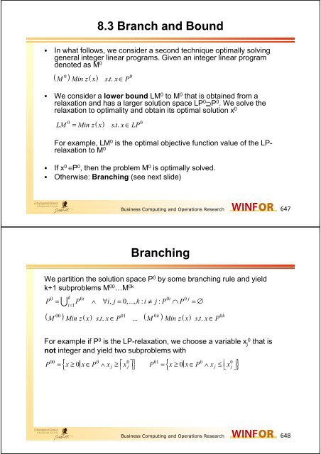
8.3 Branch and Bound
In what follows, we consider a second technique optimally solving
general integer linear programs. Given an integer linear program
denoted as M 0
( ) ( )
0 0
M Min z x s. t. x ∈ P
We consider a lower bound LM0 to M0 that is obtained from a
relaxation and has a larger solution space LP0⊇P0 . We solve the
relaxation to optimality and obtain its optimal solution x0 relaxation to optimality and obtain its optimal solution x
LM = Min z( x) s. t. x ∈ LP
0 0
For example, LM 0 is the optimal objective function value of the LPrelaxation
to M 0
If x 0 ∈P 0 , then the problem M 0 is optimally solved.
Otherwise: Branching (see next slide)
Business Computing and Operations Research 647
Branching
We partition the solution space P 0 by some branching rule and yield
k+1 subproblems M 00 …M 0k
∪
0 k 0i 0i 0 j
, 0,..., : :
i=
1
P = P ∧ ∀ i j = k i ≠ j P ∩ P = ∅
( ) ( ) ( ) ( )
00 01 0k 0k
M Min z x s. t. x ∈ P ... M Min z x s. t. x ∈ P
For example if P0 is the LP-relaxation, we choose a variable x 0 For example if P that is
0 is the LP-relaxation, we choose a variable x 0
j that is
not integer and yield two subproblems with
{ 0 j ⎡ j ⎤} { 0
j ⎢ j ⎥}
00 0 0 01 0 0
P = x ≥ x ∈ P ∧ x ≥ ⎢x ⎥ P = x ≥ x ∈ P ∧ x ≤ ⎣x ⎦
Business Computing and Operations Research 648

Enumeration tree obtained from Branching
Applying the branching rule consecutively, we derive a
solution tree
M 0
M 00 M 01
M 000 M 001 M 002
Some solutions of the subproblems may be integer.
We stop if the solution tree is explored entirely and thus,
the best known integer solution is optimal to M 0
Business Computing and Operations Research 649
Size of the enumeration tree
Hmmm… Annoying is that its
size grows exponentially!
This can take ages to
compute…
But we can reduce
the size by
bounding…
bounding… !
Business Computing and Operations Research 650

Bounding
There is always a global upper bound UM to the integer linear program
M 0 . Either UM=∞ or UM is derived from a feasible solution to M 0
We calculate a lower bound LM 0i , which is easy to calculate, for each
subproblem M 0i and LM 0i has a solution space LP 0i ⊇P 0i ∀i=1,…,k.
A subproblem M0i does not need to be considered any more (i.e., it is
pruned) if one of the following pruning criterions hold:
0i
a) and the optimal solution x0i of LM0i is feasible to M0 a) LM < UM and the optimal solution x of LM is feasible to M : We
found an improved upper bound to M0 and we remember this
solution UM:= LM0i .
b) : The optimal solution of the subproblem M0i LM < UM
0i
LM ≥ UM
and all
integer solutions derived from it cannot be better than the best
known feasible solution with UM.
0i
c) : There exists no feasible solution to LM0i and none to M0i LP = ∅
We stop if the solution tree is explored and thus, UM is optimal to M 0
( 0 )
M Minimize − x − 2 ⋅ x
s.t. 2 ⋅ x + 2 ⋅ x ≤ 7
1 2
1 2
−2 ⋅ x + 2 ⋅ x ≤ 1
1 2
−2 ⋅ x ≤ −1
x ,x
2
≥ 0
x ,x ∈Z
1 2
Business Computing and Operations Research 651
1 2
Example
We commence with UM=∞ and with the LP-relaxation LM0 0
7
1
−1
−1 2
−2
0
−2
2
2
−2
0
1
0
0
0
0
1
0
11
0 2
3
0
⇒ ... ⇒
2
0 3
1
2
0
1
0
0
0
0
0
1
3
4
1
4
1
2
1
4
1
4
− 1
4
1
2
1
4
0
0
1
0
Business Computing and Operations Research 652

Consequences
Obviously, -11/2 is a lower bound for the optimal solution
value of M 0
Since the solution is unfortunately not integer, we branch
and conduct a case statement. Either x 1≤1 or x 1≥2
Starting from the original set of feasible solutions
{ ( 1 2 ) ≥0
2 1 2 2 7 2 1 2 2 1 2 2 1 }
0 2
P = x ,x ∈ IR | 2 ⋅ x + 2 ⋅ x ≤ 7 ∧ − −2 ⋅ x + 2 ⋅ x ≤ 1 ∧ 2 ⋅ x ≤ − −1
the simple branching step yields two subproblems
{ ( 1 2 ) ≥0
2 1 2 2 7 2 1 2 2 1 2 2 1 1 1}
( ) 2 2 7 2 2 1 2 1 2
00 2
P x ,x IR | x x x x x x
= ∈ ⋅ + ⋅ ≤ ∧ − ⋅ + ⋅ ≤ ∧ ⋅ ≤ − ∧ ≤ ∧
{ 1 2 ≥0
1 2 1 2 2 1 }
= ∈ ⋅ + ⋅ ≤ ∧ − ⋅ + ⋅ ≤ ∧ ⋅ ≤ − ∧ ≥
01 2
P x ,x IR | x x x x x x
Business Computing and Operations Research 653
Resulting problems
Consequently, we obtain the tableaus
M M
00 01
11
2
0 0 3
4
1
4
0 0 11
2
0 0 3
4
1
4
0 0
3
2
1 0 1
4
− 1
4
0 0 3
2
1 0 1
4
− 1
4
0 0
3 0 0 1
2
1
2
1 0 3 0 0 1
2
1
2
1 0
2 0 1 1
4
1
2
0 0 2 0 1 1
4
1
2
0 0
1 1 0 0 0 0 1 2 1 0 0 0 0 −1
Business Computing and Operations Research 654

Transformation of the tableaus
In order to directly conduct the dual simplex, we
need to transform the problem
Specifically, we subtract the first row from the
fourth one or vice versa
Thus, we obtain
11
2
0 0 3
4
1
4
0 0 11
2
0 0 3
4
1
4
0 0
3
2
1 0 1
4
− 1
4
0 0 3
2
1 0 1
4
− 1
4
0 0
3 0 0 1
2
1
2
1 0 3 0 0 1
2
1
2
1 0
2 0 1 1
4
1
2
0 0 2 0 1 1
4
1
2
0 0
− 1
2
0 0 − 1
4
1
4
0 1 − 1
2
0 0 1
4
− 1
4
0 1
Business Computing and Operations Research 655
Finally, it turns out…
11
2
0 0 3
4
1
4
0 0 11
2
0 0 3
4
1
4
0 0
3
2
1 0 1
4
− 1
4
0 0 3
2
1 0 1
4
− 1
4
0 0
3 0 0 1
2
1
2
1 0 3 0 0 1
2
1
2
1 0
2
⎡− 1 ⎤
⎣ 2⎦ 0
0
1
0
1
4
( − 1
4) 1
4
1
4
0
0
0
1
2
⎡− 1 ⎤
⎣ 2⎦ 0
0
1
0
1
4
1
4
1
4
( − 1
4)
0
0
0
1
4 0 0 0 1 0 3 5 0 0 1 0 0 1
1 1 0 0 0 0 1 2 1 0 0 0 0 −1
2 0 0 0 1 1 2 2
3
2
0 1 0 1
2
0 1
2 0 0 1 −1 0 −4
0 0 1 0 1 2
3
2
0 1 1
2
0 0 1
2 0 0 −1 1 0 −4
Business Computing and Operations Research 656

Conclusions
Unfortunately, both solutions are still not integer
Thus, we have to resume with the next branching
step
This time, we obtain altogether four constellations
000 { ( 1 2 ) 2
≥ 0 2 1 2 2 7 2 1 2 2 1 2 2 1 1 1 2 1 }
001 { ( 1 2 ) 2
≥0
2 1 2 2 7 2 1 2 2 1 2 2 1 1 1 2 2}
010 { ( 1 2 ) 2
≥0
2 1 2 2 7 2 1 2 2 1 2 2 1 1 2 2 1}
011
= { ( 1 2 ) ∈
2
≥0
2 ⋅ 1 + 2 ⋅ x2 ≤ 7 ∧ −2 ⋅ x1 + 2 ⋅ x2 ≤ 1∧ 2 ⋅ x2 ≤ −1∧ x1 ≥ 2 ∧ x2
≥ 2}
M = x ,x ∈ IR | ⋅ x + ⋅ x ≤ ∧ − ⋅ x + ⋅ x ≤ ∧ ⋅ x ≤ − ∧ x ≤ ∧ x ≤ ∧
M = x ,x ∈ IR | ⋅ x + ⋅ x ≤ ∧ − ⋅ x + ⋅ x ≤ ∧ ⋅ x ≤ − ∧ x ≤ ∧ x ≥ ∧
M = x ,x ∈ IR | ⋅ x + ⋅ x ≤ ∧ − ⋅ x + ⋅ x ≤ ∧ ⋅ x ≤ − ∧ x ≥ ∧ x ≤ ∧
M x ,x IR | x
M 001 and M 011 are infeasible (case c)
Thus, we resume with M 000 and M 010
Business Computing and Operations Research 657
Resulting problems
M M
000 010
4 0 0 0 1 0 3 0 5 0 0 1 0 0 1 0
1 1 0 0 0 0 1 0 2 1 0 0 0 0 −1
0
2 0 0 0 1 1 2 0 2 0 0 1 0 1 2 0
3
2
0 1 0 1
2
0 1 0 3
2
0 1 1
2
0 0 1 0
2 0 0 1 −1 0 −4 0 2 0 0 −1 1 0 −4
0
1 0 1 0 0 0 0 1 1 0 1 0 0 0 0 1
4 0 0 0 1 0
3 0 5 0 0 1 0 0 1 0
1 1 0 0 0 0 1 0 2 1 0 0 0 0 −1
0
2 0 0 0 1 1 2 0 2 0 0 1 0 1 2 0
3
2
0 1 0 1
2
0 1 0 3
2
0 1 1
2
0 0 1 0
2 0 0 1 −1 0 −4 0 2 0 0 −1 1 0 −4
0
( ) ( )
− 1 0 0 0 − 1 0 −1 1 − 1 0 0 − 1 0 0 −1
1
2 2 2 2
Business Computing and Operations Research 658

Resulting problems
4 0 0 0 1 0 3 0 5 0 0 1 0 0 1 0
1 1 0 0 0 0 1 0 2 1 0 0 0 0 −1
0
2 0 0 0 1 1 2 0 2 0 0 1 0 1 2 0
3
2
0 1 0 1
2
0 1 0 3
2
0 1 1
2
0 0 1 0
2 0 0 1 −1 0 −4 0 2 0 0 −1 1 0 −4
0
( ) ( )
⎡− 1 ⎤ 0 0 0 − 1 0 −1 1 ⎡− 1 ⎤ 0 0 − 1 0 0 −1
1
⎣ 2 ⎦ 2 ⎣ 2 ⎦
2
3 0 0 0 0 0 1 2
1 1 0 0 0 0 1 0
1 0 0 0 0 1 0 2
1 0 1 0 0 0 0 1
3 0 0 1 0 0 −2 −2
1 0 0 0 1 0 2 −2
9
2
0 0 1
2
0 0 0 1
5
2
1 0 1
2
0 0 0 −1
1 0 0 0 0 1 0 2
1 0 1 0 0 0 0 1
4 0 0 1 1 0 0 −4
1 0 0 1
2 2
0 0 1 −1
Business Computing and Operations Research 659
M 000 and M 010 – Results
Obviously, the problems are optimally solved
Thus, we obtain an integer solution with objective
function value -3 from M 000 and we set UM:=-3
(case a)
Since the lower bound of the remaining problem
M010 is -9/2, we have to resume with this problem
Here, we obtain the new problems
0100 2
M { ( x 1,x 2 ) IR ≥0
| 2 x1 2 x2 7 2 x1 2 x2 1 2 x2 1 x1 2 x2 1 x1
2}
0101 2
M = { ( x 1,x 2 ) ∈ IR ≥0
| 2 ⋅ x1 + 2 ⋅ x2 ≤ 7 ∧ −2 ⋅ x1 + 2 ⋅ x2 ≤ 1∧ 2 ⋅ x2 ≤ −1∧ x1 ≥ 2 ∧ x2 ≥ 2 ∧ x1
≥
3}
= ∈ ⋅ + ⋅ ≤ ∧ − ⋅ + ⋅ ≤ ∧ ⋅ ≤ − ∧ ≥ ∧ ≤ ∧ ≤ ∧
Business Computing and Operations Research 660

M 010 – Results
M M
0100 0101
9
2
0 0 1
2
0 0 0 1 0 9
2
0 0 1
2
0 0 0 1 0
5
2
1 0 1
2
0 0 0 −1 0 5
2
1 0 1
2
0 0 0 −1
0
1 0 0 0 0 1 0 2 0 1 0 0 0 0 1 0 2 0
1 0 1 0 0 0 0 1 0 1 0 1 0 0 0 0 1 0
4 0 0 1 1 0 0 −4
0 4 0
0 1 1 0 0 −4
0
1
2
0 0 1
2
0 0 1 −1
0 1
2
0 0 1
2
0 0 1 −1
0
2 1 0 0 0 0 0 0 1 3 1 0 0 0 0 0 0 − 1
9
2
0 0 1
2
0 0 0 1 0 9
2
0 0 1
2
0 0 0 1 0
5
2
1 0 1
2
0 0 0 −1 0 5
2
1 0 1
2
0 0 0 −1
0
1 0 0 0 0 1 0 2 0 1 0 0 0 0 1 0 2 0
1 0 1 0 0 0 0 1 0 1 0 1 0 0 0 0 1 0
4 0 0 1 1 0 0 −4 0 4 0 0 1 1 0 0 −4
0
1
2
0 0 1
2
0 0 1 −1 0 1
2
0 0 1
2
0 0 1 −1
0
− 1
2
0 0 − 1
2
0 0 0 1 1 − 1
2
0 0 1
2
0 0 0 −1
1
Business Computing and Operations Research 661
And thus, we obtain
9
2
0 0 1
2
0 0 0 1 0 9
2
0 0 1
2
0 0 0 1 0
5
2
1 0 1
2
0 0 0 −1 0 5
2
1 0 1
2
0 0 0 −1
0
1 0 0 0 0 1 0 2 0 1 0 0 0 0 1 0 2 0
1 0 1 0 0 0 0 1 0 1 0 1 0 0 0 0 1 0
4 0 0 1 1 0 0 −4 0 4 0 0 1 1 0 0 −4
0
1 1 1 1
2
0 0
2
0 0 1 −1 0
2
0 0
2
0 0 1 −1
0
⎡− 1 ⎤ 0 0 ( − 1 ) 0 0 0 1 1 ⎡− 1 ⎤ 0 0 1 0 0 0 ( −1)
1
⎣ 2 ⎦ ( 2 2) ⎣ 2 ⎦ 2
( )
4
2
1
1
0
1
0
0
0
0
0
1
0
0
0
0
0
0
0
0
0
0
1
0
0
0
0
0
2
0
2
1
4
1
3
1
0
0
1
0 2
0
1
0
0
0
0
0
1
1
0
1
1
2
0
0
0
0
0
0
1
0
0
0
0
0
0
0
0
0
1
−1
2
1
3 0 0 0 1 0 0 −4 −2 6 0 0 −1 1 0 0 0 −4
0 0 0 0 0 0 1 0 1 1 0 0 0 0 0 1 0 −1
1 0 0 1 0 0 0 2 2 1 0 0 1
2
−
2
0 0 0 1 −1
Business Computing and Operations Research 662

M 0100 and M 0101 – Results
We obtained an improved second feasible
solution x T =(2,1) from M 0100 and UM:=-4 (case a)
The other alternative constellation M 0101 still does
not provide any integer solution
However, since the objective function value is -4,
this is a lower bound for all integer solutions
resulting from M0101 (case b)
Thus, we explored the solution tree and stop our
procedure. The optimal solution is x T =(2,1) with
an objective function value of UM=-4
Business Computing and Operations Research 663
Example – Conducted exploration process
00 00
( )
LM = − 4 x = 1,3/ 2
x1 ≤ 1
M 0
0 0
M 00 M 01
( )
LM = − 11/ 2 x = 3/ 2,2 UM = ∞
x1 ≥ 2
01 01
( )
LM = − 5 x = 2,3/ 2
x2 ≤ 1
x2 ≥ 2 x2 ≤ 1
x2 ≥ 2
M000 M001 M010 M011 M M M 010
x = ( 5/ 2,1 )
M
x = 5/ 2,1
LM
x
000
000
=
case a)
000
= −3
( 1,1)
case c)
001
LM < UM ⇒ UM : = −3
P = ∅
LM
010
= −9/
2
x1 ≤ 2
x1 ≥ 3
M 0100 M 0101
LM
x
0100
0100
=
case a)
0100
= −4
( 2,1)
LM < UM ⇒ UM : = −4
Optimal Solution
LM
0101
0101
case b)
0101
= −4
( 3,1/ 2)
case c)
Business Computing and Operations Research 664
x
=
LM ≥
UM
011
P = ∅

Branch and Bound Algorithm
1. Determine an upper bound UM either via a heuristic or set UM:=∞
2. Solve a lower bound LM i of M i and obtain its optimal solution x i
3. If either LM i ≥UM (case b) or P i =Ø (case c) hold, then go to 7.
4. Otherwise (Case b) or c) do not apply): If LM i