A Scenario Framework - ERM Symposium

© 2008 R 2 Financial Technologies 

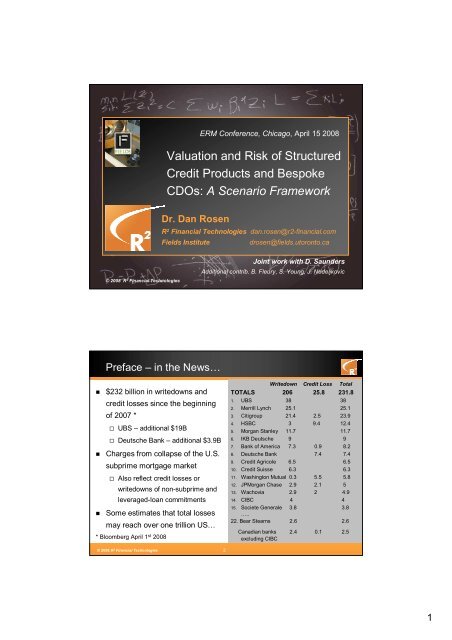
Valuation and Risk of Structured 

Credit Products and Bespoke 

CDOs: A Scenario Framework 

Dr. Dan Rosen 

R 2 Financial Technologies dan.rosen@r2-financial.com 

Fields Institute drosen@fields.utoronto.ca 

Preface – in the News… 

$232 billion in writedowns and 

credit losses since the beginning 

of 2007 * 

UBS – additional $19B 

Deutsche Bank – additional $3.9B 

Charges from collapse of the U.S. 

subprime mortgage market 

Also reflect credit losses or 

writedowns of non-subprime and 

leveraged-loan commitments 

Some estimates that total losses 

may reach over one trillion US… 

* Bloomberg April 1 st 2008 

© 2008 R 2 Financial Technologies 2 

ERM Conference, Chicago, April 15 2008 

Joint work with D. Saunders 

Additional contrib. B. Fleury, S. Young, J. Nedeljkovic 

Writedown Credit Loss Total 

TOTALS 206 25.8 231.8 

1. UBS 38 38 

2. Merrill Lynch 25.1 25.1 

3. Citigroup 21.4 2.5 23.9 

4. HSBC 3 9.4 12.4 

5. Morgan Stanley 11.7 11.7 

6. IKB Deutsche 9 9 

7. Bank of America 7.3 0.9 8.2 

8. Deutsche Bank 7.4 7.4 

9. Credit Agricole 6.5 6.5 

10. Credit Suisse 6.3 6.3 

11. Washington Mutual 0.3 5.5 5.8 

12. JPMorgan Chase 2.9 2.1 5 

13. Wachovia 2.9 2 4.9 

14. CIBC 4 4 

15. Societe Generale 3.8 3.8 

….. 

22. Bear Stearns 2.6 2.6 

Canadian banks 2.4 0.1 2.5 

excluding CIBC 

1

Preface – in the News… 

Investors blaming a “1 in 10,000 years” event… 

And then… 

“It all happened exactly like he said it would happen... In every single 

detail…” 

“The hedge fund creator's name was John Paulson… by making 

between $3 billion and $4 billion for himself in 2007, he 

appears to have set a Wall Street record… no one has ever 

made so much so fast.” 


Sources: Reuters, Risk, Banking Technology,, Dow Jones, FT,, G&M, Bloomberg 

Structured Credit – Valuation & Risk 

1. Lack of integrated view of synthetic and cash products and single-name 

credit derivatives: pricing and risk management 

2. Valuation of synthetic CDOs 

Gaussian copula framework still prevalent 

Pricing bespoke portfolios difficult – “mapping” models are generally ad-hoc 

Dynamic models and detailed bespooke models still in infancy 

3. Valuation of structured credit (cash CDOs, ABSs,…) 

Difficult, non-standard, computationally intensive 

IR, spreads, prepayment, credit (and correlation) risks 

Structures are complex and opaque 

Simple “bond models” and matrix pricing generally used – pricing based on 

ratings 

Advanced models are fairly new or not fully developed for all asset classes 

Standardized calibration is difficult to achieve 


2

Structured Credit – Valuation & Risk 

4. Risk modelling is immature (market and credit risk) 

Simple market risk sensitivities are generally used (e.g. CR01, etc.) 

Risk assessment and investment decision mainly driven by ratings 

VaR (market & credit) measures not easy to obtain and not used in general 

Risk contribution not well defined (non-linearities) 

Hedging has proven to be difficult and prone to large model errors 

Computationally intensive risk applications (e.g. name-specific sensitivities) 

Correlation is very important but difficult to assess 

High systematic risk 


Summary 

Scenario framework – Valuation and Risk Profiling 

Implied factor distributions and weighted MC techniques 

Multi-factor credit models – characterize correlations for different baskets 

Weighted Monte Carlo techniques (used in options pricing) 

CDO analytics and computational techniques 

Ability to incorporate a full bottom-up approach 

Basic idea: set of scenarios where instruments are consistently valued 

Imply “risk-neutral” distribution (process) for underlying systematic risk factors 

Observed (liquid) prices (e.g. CDSs, index tranches) 

Prior or “quality” preferences on distribution; subjective views 

Structured finance CDOs (ABS and CLO products) 

Flexibly incorporate cash-flow waterfalls, prepayment and LGD models 

Cash CDO = bespoke portfolio + complex cashflow waterfall 

Methodology is general (dynamic) – examples in paper use static models 


3

PART 1 

Introduction: Valuing CDOs 


Synthetic CDOs 


and Structured Credit 

Underlying pool of credit default swaps – divided into “tranches” 

Tranche 

Equity 

1st Mezzanine 

2nd Mezzanine 

Senior 

Super Senior 

L , 

n j 

Attachment 

0% 

3% 

7% 

10% 

15% 

Detachment 

3% 

7% 

10% 

15% 

30% 

Size of the n-th tranche 

S = U N − A N = N ⋅ U − A ) 

n 

n 

Cumulative portfolio loss of up to t j 

∑ N k ⋅ LGDk 

⋅ 

k ≤t 

1 

L τ 

j = 

j 

k 

L = min( S , max( L − A 

n, 

j 

n 

j n 

n 

( n n 

Cumulative loss on the n-th tranche up to time tj 

A U 

n = An 

+ 1 

n 

L j 

, 0)) 

4

Background – Pricing Synthetic CDOs 

Standard model for pricing synthetic CDOs: single-factor Gaussian 

copula (Li 2001) 

Codependence through a one-factor Gaussian copula of times to default 

Single parameter to estimate (correlation for all obligors in portfolio) 

Basic model does not simultaneously match market prices of all traded 

tranches 

“Correlation skew” – set of correlations that match the prices of all tranches 

Base correlations – alternative to tranche correlations 

Implied correlations of equity tranches with different attachment points 

(mezzanine/senior tranches as difference between two equity tranches) 

Interpolation (or extrapolation) model 

Calibrated to observed tranche prices (e.g iTraxx or CDX) 

Pricing of bespoke portfolios – mapping (risk of bespoke vs. index portfolio) 


Single-Factor Gaussian Copula (Times to Default) 

Cumulative default time 

distribution functions 

Creditworthiness index 

Z systematic factor (Gaussian) 

Default times 

Mapping to Gaussian 

Conditional on Z, default times 

are independent 

∑ 

Explicit formulae for conditional 

default probabilities 


( τ ) ⋅ LGD ( ) 

L 1 ⋅V 

τ 

k 

T = τ ≤T 

k 

k 

k 

k 

k 

k 

−1 

k 

τ = F Φ 

( ( Y ) ) 

Z 

( t) 

= Pr( 

τ ≤ t Z ) q ( t) 

= Pr( 

τ > t Z ) 

Z 

pk k 

j 

k 

p 

Z 

k 

( t) 

Y = ρ Z + 1− 

ρ ε 

k 

Fk k 

⎛ Φ 

= Φ⎜ 

⎜ 

⎝ 

( t) 

= Pr( τ ≤ t) 

k 

( F ( t) 

) ⇔ τ ≤ t 

Yk ≤ Φ k 

k 

−1 

−1 

( F ( t) 

) 

k 

k 

k 

− ρ ⎞ k Z 

⎟ 

1− 

ρ ⎟ 

k ⎠ 

k 

5

General Framework: Gaussian Copula Model 

1. Scenarios: 

systematic 

factors 

Z 

p 

2. Conditional 

def. prob. 

Z 

k 

( t) 

= 

⎛ 

⎜ 

Φ 

Φ 

⎜ 

⎝ 

( F ( t) 

) 

− ρ ⎞ 

k Z 

⎟ 

1− 

ρ ⎟ 

k ⎠ 



−1 

k 


portfolio losses 

(discounted) 

Conditionally independent obligor losses 

convolution methods: 

Recursions (Andersen et al, Hull-White) 

Full simulation (independent Bernoulli 

variables) 

LLN, or CLT approximation 

Poisson approximation 

L 

( Z ) = ∑ Nk 

⋅ LGDk 

( Z ) ⋅ τ t ( Z ) 

k ≤ 1 

j j 

k 

General Framework: Gaussian Copula Model 


systematic 

factors 

Z 

p 


def. prob. 

Z 

k 

( t) 

= 

⎛ 

⎜ 

Φ 

Φ 

⎜ 

⎝ 

−1 

( F ( t) 

) 

k 

− ρ ⎞ 

k Z 

⎟ 

1− 

ρ ⎟ 

k ⎠ 

L , 

n j 



(discounted) 

Conditional 

tranche losses 

L = min( S , max( L − A 

n, 

j 

n 

j n 

A U 

n = An 

+ 1 

n 

, 0)) 

L j 

6

General Framework: Implied Factor Distributions 


systematic 

factors 

Z 


def. prob. 

p 

Z 

k 

( t) 

= 

⎛ Φ 

Φ⎜ 

⎜ 

⎝ 

( F ( t) 

) 

− ρ ⎞ j Z 

⎟ 

1− 

ρ ⎟ 

j ⎠ 


−1 

Calibration: 

k 

Correlation of 

each tranche j 

Base correlation 

Equity tranches 




(discounted) 

Bespoke Portfolios and Mappings 

0.8 

0.6 

0.4 

0.2 

0 

Conditional 


Base Correlation (Poisson) 

4. Expected tranche 

losses & values 

+ 

+ 

0 - 3% 0 - 7% 0 - 10% 0 - 15% 0 - 30% 

CDXIG5YR CDXIG7YR CDXIG10YR 

Conditional 

value of 

tranches 

. . . 

______ 

∑ 

ω ∑ p 

ω ∑ pω 

ω 

pω 

E[ 

V | Zω 

] 

ω E[ 

V | Zω 

] 

E[ 

V | Z ] 

Main idea: base correlations correspond to different levels of risk in the 

reference portfolio 

By finding the same risk levels on the bespoke portfolio – transfer the base 

correlation structure from the standard portfolio to the bespoke 

Generally, solve an equation of the form: 

S is a "risk statistic"; P the portfolio, u the detachment point), and rho is 

the base correlation (the unknown is ). 

Mapping: solve for the detachment point(s) in the bespoke portfolio 

which matches the equation: 

S ( Pˆ 

, uˆ 

, ρ) = S( 

P, 

u, 

ρ) 

Note: the base correlation for the standard portfolio is used on both sides 

û 

ω 

7

EL Mapping (Base Correlations) 

ρ(U) 

3% 7% 10% 15% 30% U 


Index Base Correlation Curve 

Bespoke Base Correlation Curve 

Understanding Bespoke Portfolios and Prices 

Differences in prices from bespoke portfolio and quoted (index) 

prices may arise from differences in 

Credit quality (individual names spreads/PDs) 

Concentration risk (sector/geographical, and name concentration) 

Sector concentration (indices are well diversified) 

Correlation (codependence) 

Granularity 

Reference to multiple indices (and different risk premia) 

Liquidity 

e.g. for an equity tranche: 

Higher quality (lower individual spreads) lower tranche spread 

Higher correlation lower spread 

Higher granularity (more names) higher spread 

Multiple indices lower average correlation higher spread 


8

Cash CDOs: “Bond” Models (Single-Scenario) 

Defaults 

Recoveries 

Prepayments 

Collateral 

Model 

Collateral 

Cash Flows 

Step 1: Gather collateral cash flow assumption 

vectors 

e.g. assumptions by type of CDO collateral (e.g. CRE, 

ABS, loan, bond) 

For ABS CDOs, can use loan performance analysis on 

the loans in each ABS 

Step 2: Generate cash flows for each piece of 

collateral 

CDO Model 


Senior Cash Flow 

Mezz Cash Flow 

Junior Cash Flow 

Equity Cash Flow 

Step 3: Use collateral CFs and CDO waterfall to 

generate CDO cash flows 

Step 4: NPV – discount cash flows (appropriate 

discount rate) 

Complex cashflow from collateral and structure waterfall 

Discount 

Discount 

Discount 

Discount 

Price 

Price 

Price 

Price 

Discount rate (spread) – from market quotes where available 

Application of discount rate to all other tranches with the 

same rating, deal type, vintage, etc. 

In addition to default, LGDs: prepayment (applies differently to tranches) 

Underlying: loans, bonds, retail loans (mortgages, credit cards, etc.), ABSs, CDOs 

(CDO^2) 

Cash CDOs: “Bond” Models (Single-Scenario) 

Single-scenario modelling 

Deterministic cash-flow approach (scheduled amortization) 

No direct modelling of correlations, optionality, non-linearities 

Detailed cash-flow modelling of collateral pool and of CDO waterfall 

Pool level assumptions and loan-level assumptions and clustering 

Comparative pricing via matrix approach (generally relies on ratings) 

Scenario assumptions, discount spreads (premiums) 

Useful stress-testing framework 

PV 

( Y ) 


T 

∑ 

= 

j= 

1 

CF 

j 

⋅ e 

−( 

r + s ( X ) ) ⋅t 

( PP, 

Def , LGD,... 

) = ( rating, sector, vintage, ... ) 

Y 

= X 

j 

j 

9

PART 2 

Scenario Framework: 

Implied Factor Distributions 

and Weighted Monte Carlo Methods 


Credit Risk and Multi-Factor Models 

Multi-factor models are currently used extensively to asses portfolio 

credit risk and measure credit economic capital 

Capital allocation – capture sector/geographical concentrations 

Over a decade of industry experience: KMV, CreditMetrics, 

CreditRisk+, CreidtPortfolioView 

Conditional independence framework – mathematical equivalence 

Extensive empirical studies on estimation of credit correlation 

parameters (Basel committee, rating agencies, vendors, financial 

institutions and academics) 

The origins of the Gaussian copula method to price CDOs trace back 

to the KMV and CreditMetrics model 


10

Implied Factor Models & Weighted MC 

Background 

Weighted MC approach used to price complex options 

e.g. Avellaneda et al., 2001, Elices and Giménez, 2006 

Similar idea to fitting the implied distribution (or process) of 

underlying in a (discrete) lattice 

Hul-White’s “implied copula” model (2006) is essentially an 

application of this concept 

Homogeneous portfolio – cannot be used directly to price bespokes 

Similar ideas (also for homogeneous portfolios) in Brigo et al (2006), 

Torresetti et al (2006) 


Implied Factor Models & Weighted MC 

Assumptions 

Correlations of names in portfolio: multi-factor model (systematic factors) 

MF model joint default behaviour under real world measure P 

Coefficients of factor model for portfolio are known and fixed 

Difference between real measure P and RN-measure Q : joint 

distribution of the systematic factors 

(Marginal) distribution of default times for each name under the risk-neutral 

measure based on CDS spreads 

Conditional distribution of default times, as a function of the factor levels 

under the RN measure still given by the same formula 

Solution 

Sample discrete “paths” (in this case, single values) for the systematic 

factors and adjust probabilities of paths to match prices 


11

Weighted MC – GLLM Framework 

Portfolio model can be a Gaussian copula or, more generally, we 

can use other “link functions” 

Logit, NIG, double-t, etc… 

Generalized linear mixed models (GLMM) 

Example of general multi-factor copula 

Match, for each name, the “unconditional” default probability term 

structure 

p 

( t) 

= h a( 

t) 

Z ( t) 

= p ( t) 

df ( z) 

… and match quoted CDO prices 


Z 

j 

p 

j ∫ 

( −∑ 

bk 

Zk 

) 

Weighted MC – GLLM Framework 

General formulation: 

Gaussian copula: 

a 

Logit model: 

it 

= 

t 

PD ( Z ) = h 

−1 

1− 


Φ 

it 

( PD ) 

it 

, 

j 

k 

p 

Z 

j 

K t t 

( ait 

+ bik 

Zk 

) 

b 

∑ k = 

K 2 

K 

∑ β 

− 

k = k 1 

1 ∑k 

= 

Poisson mixture (e.g. CreditRisk+) 

ik 

= 

K 

∑ k = 1 

1 

h( 

x) 

= 

( 1+ 

exp( −x)) 

β 

λ 

( Z) 

= E[ 

U | Z] 

= c β Z 

i 

i 

i 

ik 

1 

k 

k 

β 

2 

1 k 

( t) 

⎛ 

⎜ H 

= G j ⎜ 

⎝ 

−1 

( Fj 

( t) 

) −∑ 

−∑ 

β ⎞ 

k k Zk 

⎟ 

1 

2 

β k k 

⎟ 

⎠ 

12

General Framework: Weighted MC 


systematic 

factors 

q1 

q2 

q3 

Objective function (e.g. max. 

smoothness, max entropy, etc.) 

∑ 

ω ∑ ω p 

ω 

pωE[ 

V | Zω 

] = 0 

pω 

E[ 

V | Zω 

] = 0 

E[ 

V | Z ] = 0 

ω 

Z 

ω 

p 


def. prob. 

Z 

j 

( t) 

= 

⎛ Φ 

Φ⎜ 

⎜ 

⎝ 

5. Optimization 

? 

( F ( t ) ) 

− ρ ⎞ k Z 

⎟ 

1− 

ρ ⎟ 

k ⎠ 


−1 

j 



(discounted) 

Global Factor Implied Distribution 

Conditional 


4. Expected tranche 

losses & values 

Evolution of distribution – from prior to tight fit of prices 


+ 

+ 

Conditional 

value of 

tranches 

. . . 

______ 

∑ 

ω ∑ p 

ω ∑ pω 

ω 

pω 

E[ 

V | Zω 

] 

ω E[ 

V | Zω 

] 

E[ 

V | Z ] 

ω 

13

Implied Factor Distributions – Intuition 

Key objective: tractable distribution of joint default times – match 

marginal distributions and prices of CDSs and quoted CDO tranches 

In a Gaussian copula – conditioning on the systemic factor 

( t) 

⎛ Φ 

= Φ⎜ 

⎜ 

⎝ 

−1 

( F ( t) 

) 


p 

Z 

j 

j 

− ρ Z ⎞ 

⎟ 

1− 

ρ ⎟ 

⎠ 

Base correlations the correlation rho is a function of the 

detachment point 

Implied copula model directly conditional PDs through discrete 

scenarios (on a hazard rate) for homogeneous portfolio 

Implied multi-factor distribution model directly the distribution of 

the systematic risk factor through discrete scenarios conditional 

default probabilities through the copula “mapping” 

Extensible to multi-factor and applied to other portfolios 

Weighted MC – Optimization problem 

Objective function factor distribution “quality”: 

min. distance from prior, max. entropy, max. smoothness 

Match tranche and index prices (can be more than one index at a time) 

Match CDS prices (cumulative default probabilities for all names) 

max G( 

q) 

M 

m 

n m 

( Z ) = ∑q 

mPV 

Sell ( Z ) 

Trade-off: well-behaved “smooth” solution might be preferred over 

perfect matching of prices (with some bounds) 

Instead of perfect “perfect match” – minimize price differences 


M 

∑ 

M 

M 

q 

m 

m= 

1 

∑ 

q 

m 

m= 

1 

∑ 

q 

m 

m= 

1 

PV 

PD 

n 

Buy 

i, 

j 

= 1 , 

subject to : 

m 

( Z ) = F 

q 

m 

m= 

1 

i, 

j 

≥ 0 

for all i, 

j 

for all 

m 

for all 

n 

14

Weighted MC – Computation 

Computational issues 

Each path requires computing the conditional portfolio loss 

distribution – trade-off between number of paths and accuracy of 

these distributions 

Number of paths 

Low dimensions – numerical integration 

More generally – Quasi-MC methods (low discrepancy 

sequences) 

Trade-off: nice behaved “smooth” solution might be preferred over 

perfect matching of prices (with some bounds of course) 


Weighted MC – Scenario Generation 

Quasi Monte Carlo methods 

Deterministic points generated from 

a type of mathematical vector 

sequences: low discrepancy 

sequences (LDS) 

Basic idea: 

LDSs specifically attempt to cover 

the space of risk factors “evenly” - 

avoiding the clustering usually 

associated with pseudo-random 

sampling 

Number of scenarios necessary to 

achieve a desired level of accuracy 

in pricing or risk calculations is 

reduced 


Source: Dembo et al. (1999), Mark-to-Future 

15

PART 3 


Examples 

1. ABX and cash CDO 

2. CLO and HY Index 

Examples 

3. Bespoke synthetic CDO in Multi-factor model (sector 

concentrations) 

4. Bespoke synthetic CDO with names in Europe and NA 

(two indices) 


16

Example 1 – ABX 

ABX –referencing 20 Asset Backed CDS (ABCDS) 

Home Equity / Sub-prime Bonds (thousands of small loans) 

Five indices: AAA / AA / A / BBB / BBB- 

Trading Began January 2006 

Standard prices and quotes 

Modelling issues 

Default risk and prepayment risk 

Cash-flow generation 

(underlying loans, bond (and CDS) waterfall 

Defaults 

LGD/recoveries 

Prepayments 

Other factors 

Collateral 

cash-flow 

engine 



Collateral 

Cash Flows 

Example – ABX Valuation Model 

Simple valuation model (illustration purposes) 

Single systematic factor – drives 

Default rates 

Prepayment rates 

Recovery rates 

(underlying loans in the pools) 

Large homogeneous 

portfolio assumption 

Discretization 

90.00% 

80.00% 

70.00% 

60.00% 

50.00% 

40.00% 

30.00% 

20.00% 

135 systematic factor 

10.00% 

scenarios 0.00% 

ABX MktPrice 

ABX-XHAAA72_INDEX 91.81 

ABX-XHAA72_INDEX 71.06 

ABX-XHA72_INDEX 44.31 

ABX-XHBBB72_INDEX 26 

ABX-XHBBBM72_INDEX 23 

CDO 

waterfall 

p 

Z 

j 

( t) 

= h a( 

t) 

Senior tranche 

Mezz tranche 

Junior tranche 

Equity tranche 

( −∑ 

b ) k k Z k 

1 

6 

11 

16 

21 

26 

31 

36 

41 

46 

51 

56 

61 

66 

71 

76 

81 

86 

91 

96 

101 

106 

111 

116 

121 

126 

131 

PD LGD PP 

17

Example – ABX Valuation under Scenarios 

ABX bonds discounted Cashflows (values) under scenarios 

ABX MktPrice 

ABX-XHAAA72_INDEX 91.81 

ABX-XHAA72_INDEX 71.06 

ABX-XHA72_INDEX 44.31 

ABX-XHBBB72_INDEX 26 

ABX-XHBBBM72_INDEX 23 

90.00% 

80.00% 

70.00% 

60.00% 

50.00% 

40.00% 

30.00% 

20.00% 

10.00% 

$160.00 

$140.00 

$120.00 

$100.00 

$80.00 

$60.00 

$40.00 

$20.00 

$0.00 

1 

6 



0.00% 

11 

16 

21 

26 

31 

36 

41 

46 

1 

5 

9 

13 

17 

21 

25 

29 

33 

37 

41 

45 

49 

53 

57 

61 

65 

69 

73 

77 

81 

85 

89 

93 

97 

51 

56 

PD LGD PP 

71 

76 

81 

86 

91 

96 

101 

106 

111 

116 

121 

126 

131 

61 

66 

ABX-XHAAA72_INDEX ABX-XHAA72_INDEX ABX-XHA72_INDEX 

ABX-XHBBB72_INDEX ABX-XHBBBM72_INDEX 

Example – ABX Valuation and Calibration 

Example: 

Weighted MC implied factor distribution (implied scenario weights) 

Vasicek PD distribution 

(Gaussian copula GLLM) 

Implied avg. PD = 12% 

90.00% 

80.00% 

70.00% 

60.00% 

50.00% 

40.00% 

30.00% 

20.00% 

10.00% 

$20.00 

Implied correlation = 7% $0.00 

Market Price Estimated Prices 

ABX-XHAAA72 91.81 103.06 

ABX-XHAA72 71.06 94.40 

ABX-XHA72 44.31 78.89 

ABX-XHBBB72 26 57.19 

ABX-XHBBBM72 23 48.47 

0.00% 

$160.00 

$140.00 

$120.00 

$100.00 

$80.00 

$60.00 

$40.00 

2.5 0% 

2.0 0% 

1.5 0% 

1.0 0% 

0.5 0% 

0.0 0% 

1 

5 

1 

9 

6 

11 

13 

17 

16 

21 

26 

31 

36 

41 

1 

5 

9 

13 

17 

21 

25 

29 

33 

37 

41 

45 

49 

53 

57 

61 

65 

69 

73 

77 

81 

85 

89 

93 

97 

46 

51 

56 

PD LGD PP 

61 

66 

ABX-XHAAA72_INDEX ABX-XHAA72_INDEX ABX-XHA72_INDEX 

ABX-XHBBB72_INDEX ABX-XHBBBM72_INDEX 

21 

25 

29 

33 

37 

41 

45 

49 

53 

57 

61 

65 

69 

73 

77 

81 

71 

76 

81 

86 

91 

96 

101 

106 

101 

105 

109 

113 

117 

121 

125 

129 

133 

111 

101 

105 

109 

113 

117 

121 

125 

129 

133 

85 

89 

93 

97 

101 

105 

109 

113 

117 

121 

125 

129 

116 

121 

126 

131 

18

0.4 

0.35 

0.3 

0.25 

0.2 

0.15 

0.1 

0.05 

0 

0.045 

0.04 

0.035 

0.03 

0.025 

0.02 

0.015 

0.01 

0.005 

0 

1.60% 

1.40% 

1.20% 

1.00% 

0.80% 

0.60% 

0.40% 

0.20% 

0.00% 

Example – ABX Valuation and Calibration 

1 

5 

9 

13 

17 

21 

25 

29 

33 

37 

41 

45 

49 

53 

57 

61 

65 

69 

73 

77 

81 

85 

89 

93 

97 

101 

105 

109 

113 

117 

121 

125 

129 

133 

1 

5 

9 

13 

17 

21 

25 

29 

33 

37 

41 

45 

49 

53 

57 

61 

65 

69 

73 

77 

81 

85 

89 

93 

97 

101 

105 

109 

113 

117 

121 

125 

129 

133 

1 

5 

9 

13 

17 

21 

25 

29 

33 

37 

41 

45 

49 

53 

57 

61 

65 

69 

73 

77 

81 

85 

89 

93 

97 

101 

105 

109 

113 

117 

121 

125 

129 


Example – Valuing ABS CDO 

Four Steps 


Market Price Model Prices 

ABX-XHAAA72_INDEX 91.81 97.66 5.99% 

ABX-XHAA72_INDEX 71.06 69.91 -1.65% 

ABX-XHA72_INDEX 44.31 44.69 0.86% 

ABX-XHBBB72_INDEX 26 25.84 -0.63% 

ABX-XHBBBM72_INDEX 23 23.02 0.08% 

Market Price Model Price 

ABX-XHAAA72_INDEX 91.81 98.46 7.2% 

ABX-XHAA72_INDEX 71.06 69.59 -2.1% 

ABX-XHA72_INDEX 44.31 44.94 1.4% 

ABX-XHBBB72_INDEX 26 26.04 0.2% 

ABX-XHBBBM72_INDEX 23 22.70 -1.3% 

7.8% 

Market Price Model Price 

ABX-XHAAA72 91.81 101.46 10.5% 

ABX-XHAA72 71.06 69.07 -2.8% 

ABX-XHA72 44.31 45.35 2.3% 

ABX-XHBBB72 26 27.21 4.7% 

ABX-XHBBBM72 23 21.70 -5.7% 

13.3% 

1. Factor scenarios PD, PP, LGD scenarios for new CDO (factor models) 

2. CDO PV scenarios from cash-flow and waterfall engines 

3. Valuation using pre-calibrated model 

90 .00 % 

80 .00 % 

70 .00 % 

60 .00 % 

50 .00 % 

40 .00 % 

30 .00 % 

20 .00 % 

10 .00 % 

0 .00 % 

ABX PD, PP, LGD 

1 

6 

1 1 6 

2 1 

2 6 

3 1 

3 6 

4 1 

4 6 

5 1 

5 6 

6 1 

6 7 1 

7 6 

8 1 

8 6 

9 1 

9 6 

1 0 1 

1 0 6 

1 1 6 

1 2 1 

1 2 6 

1 3 1 

PD L GD PP 

90.00% 

80.00% 

70.00% 

60.00% 

50.00% 

40.00% 

30.00% 

20.00% 

10.00% 

0.00% 

CDO PD, PP, LGD 

1 

6 

1 1 

1 6 

2 1 

2 6 

3 1 

3 6 

4 1 

4 6 

5 1 

5 6 

6 1 

6 6 

7 1 

7 6 

8 1 

8 6 

9 1 

9 6 

10 1 

10 6 

11 1 

11 6 

12 1 

12 6 

13 1 

PD LGD PP 

4. Sensitivities and risk measures 

5. Model risk assessment 

$ 160.00 

$ 140.00 

$ 120.00 

$ 100.00 

“Plausible” factor distributions 

PD, PP, LGD model assumptions 

Stress testing and extreme scenarios 

$80.00 

$60.00 

$40.00 

$20.00 

$0.00 

1 

6 

11 

16 

21 

26 

31 

36 

41 

46 

51 

56 

61 

66 

71 

76 

81 

86 

91 

96 

1 01 

1 06 

1 11 

1 16 

1 21 

1 26 

1 31 

ABX-XHAAA72_IND EX ABX-XHAA72_INDEX ABX-XHA72 _INDEX 

ABX-XHBBB72_IND EX ABX-XHBBBM72_ INDEX 

0.035 

0.03 

0.025 

0.02 

0.015 

0.01 

0.005 

0 

1 

5 

9 

13 

17 

21 

25 

29 

33 

37 

41 

45 

49 

53 

57 

61 

65 

69 

73 

77 

81 

85 

89 

93 

97 

1 01 

1 05 

1 09 

1 13 

1 17 

1 21 

1 25 

1 29 

1 33 

90.00 % 

80.00 % 

70.00 % 

60.00 % 

50.00 % 

40.00 % 

30.00 % 

20.00 % 

10.00 % 

0.00% 

0.4 

0.35 

0.3 

0.25 

0.2 

0.15 

0.1 

0.05 

0 

X 

1 

6 

11 

16 

21 

26 

31 

36 

41 

46 

51 

56 

61 

66 

71 

76 

81 

86 

91 

96 

101 

106 

111 

116 

121 

126 

131 

PD L GD PP 

0.035 

0.03 

0.025 

0.02 

0.015 

0.01 

0.005 

0 

1 

5 

9 

1 3 

1 7 

2 1 

2 5 

2 9 

3 3 7 

4 1 

4 5 

4 9 

5 3 

5 7 

6 1 

6 5 

6 9 

7 3 

7 8 1 

8 5 

8 9 

9 3 

9 7 

10 1 

10 5 

10 9 

11 3 

11 7 

12 1 

12 5 

12 9 

13 3 

$1 60.00 

$1 40.00 

$1 20.00 

$1 00.00 

$8 0.00 

$6 0.00 

$4 0.00 

$2 0.00 

$ 0.00 

Best fitted 

prices 

Smoothed 

distribution 

(nonparametric) 

Optimal 

parametric 

Distribution 

PD=16.5 

R=7% 

1 

5 

9 

13 

17 

21 

25 

29 

33 

37 

41 

45 

49 

53 

57 

61 

65 

69 

73 

77 

81 

85 

89 

93 

97 

1 01 

1 05 

1 09 

1 13 

1 17 

1 21 

1 25 

1 29 

1 33 

1.80% 

1.60% 

1.40% 

1.20% 

1.00% 

0.80% 

0.60% 

0.40% 

0.20% 

0.00% 

1 

6 

11 

16 

21 

26 

31 

36 

41 

46 

51 

56 

61 

66 

71 

76 

81 

86 

91 

96 

1 01 

1 06 

1 11 

1 16 

1 21 

1 26 

1 31 

A BX -XHA AA 72_INDE X A BX -X HA A72 _INDEX A BX -X HA 72_INDE X 

A BX -XHB BB 72_INDE X A BX -X HB BB M72_INDE X 

1 

5 

9 

13 

17 

21 

25 

29 

33 

37 

41 

45 

49 

53 

57 

61 

65 

69 

73 

77 

81 

85 

89 

93 

97 

1 01 

1 05 

1 09 

1 13 

1 17 

1 21 

1 25 

1 29 

19

Example 2 – CLO Valuation 

Tranche Price 

A1 $ 101.02 

A2 $ 90.97 

B $ 77.16 

C $ 67.01 

D $ 70.77 

120.00% 

100.00% 

0.045 

80.00% 

60.00% 

40.00% 

20.00% 

0.04 

0.035 

0.03 

0.025 

0.02 

0.015 

0.01 

0.005 

0.00% 

0 

-5 

Conditional PD, LGD, and PP (on factor Z) 

-5.00 

-4.60 

-4.20 

-3.80 

-3.40 

-3.00 

-2.60 

-2.20 

-1.80 

-1.40 

-1.00 

-0.60 

-0.20 

0.20 

0.60 

1.00 

1.40 

1.80 

2.20 

2.60 

3.00 

3.40 

3.80 

4.20 

4.60 

5.00 

Loss Given Default Average Conditional 

PD (@5y) 

Factor Distribution 

Average Conditional 

PP (@5y) 

-4.6 

-4.2 

-3.8 

-3.4 

-3 

-2.6 

-2.2 

-1.8 

-1.4 

-1 

-0.6 

-0.2 

0.2 

0.6 

1 

1.4 

1.8 

2.2 

2.6 

3 

3.4 

3.8 

4.2 

4.6 

5 


Example – CLO Valuation 

Tranche Price Price 

A1 $ $ 101.02 76.60 

A2 $ $ 90.97 67.24 

B $ $ 77.16 43.32 

C $ $ 67.01 22.50 

D $ $ 

70.77 23.81 

120.00% 

100.00% 

0.045 

80.00% 

60.00% 

40.00% 

20.00% 

0.04 

0.035 

0.03 

0.025 

0.02 

0.015 

0.01 

0.005 

0.00% 

0 

-5 

Conditional PD, LGD, and PP (on factor Z) 

-5.00 

-4.60 

-4.20 

-3.80 

-3.40 

-3.00 

-2.60 

-2.20 

-1.80 

-1.40 

-1.00 

-0.60 

-0.20 

0.20 

0.60 

1.00 

1.40 

1.80 

2.20 

2.60 

3.00 

3.40 

3.80 

4.20 

4.60 

5.00 

Loss Given Default Average Conditional 

PD (@5y) 

Factor Distribution 

Average Conditional 

PP (@5y) 

-4.6 

-4.2 

-3.8 

-3.4 

-3 

-2.6 

-2.2 

-1.8 

-1.4 

-1 

-0.6 

-0.2 

0.2 

0.6 

1 

1.4 

1.8 

2.2 

2.6 

3 

3.4 

3.8 

4.2 

4.6 

5 


Conditional Tranche Values 

40 

35 

30 

25 

20 

15 

10 

5 

0 

Conditional Tranche Values 

40 

35 

30 

25 

20 

15 

10 

5 

0 

140 

120 

100 

80 

60 

40 

20 

-5.00 

-4.50 

-4.00 

-3.50 

Tranche values across factor scenarios (mean) 

0 

-5 -4 -3 -2 -1 0 1 2 3 4 5 

140 

120 

100 

80 

60 

40 

20 

-5.00 

-4.50 

-4.00 

-3.50 

Tranche prices across systematic factor (sigma) 

-3.00 

-2.50 

-3.00 

-2.50 

-2.00 

-1.50 

-2.00 

-1.50 

-1.00 

-0.50 

-1.00 

-0.50 

Factor 

0.00 

0.50 

0.00 

0.50 

1.00 

1.50 

1.00 

1.50 

2.00 

2.50 

2.00 

2.50 

3.00 

3.50 

3.00 

3.50 

4.00 

4.50 

Tranche values across factor scenarios (mean) 

0 

-5 -4 -3 -2 -1 0 1 2 3 4 5 

Factor 

Tranche prices across systematic factor (sigma) 

4.00 

4.50 

5.00 

5.00 

A1 

A2 

B 

C 

D 

A1 

A2 

B 

C 

D 

A1 

A2 

B 

C 

D 

A1 

A2 

B 

C 

D 

20

Example 3: Multi-Factor Model & Bespoke Synthetic 

Industry concentration by Notional 

CDX HY CDX IG ITRAXX EUR ITRAXX CJ ITRAXX ASIA 

Exposure Per Name 10MM 8MM 8MM 20MM 1B 

Number of Names 100 125 125 50 50 

Industry (Fitch) 

Aerospace & Defence 3.00% 4.00% 2.40% 

Automobiles 9.00% 7.20% 4.00% 4.00% 

Banking & Finance 3.00% 17.60% 20.00% 20.00% 24.00% 

Broadcasting/Media/Cable 7.00% 8.00% 7.20% 

Business Services 4.00% 1.60% 10.00% 

Building & Materials 4.00% 3.20% 4.00% 6.00% 

Chemicals 6.00% 3.20% 4.80% 2.00% 2.00% 

Computers & Electronics 10.00% 4.00% 1.60% 8.00% 6.00% 

Consumer Products 5.00% 3.20% 3.20% 4.00% 

Energy 10.00% 4.80% 1.60% 10.00% 

Food, Beverage & Tobacco 4.00% 5.60% 7.20% 4.00% 

Gaming, Leisure & Entertainment 3.00% 1.60% 0.00% 2.00% 

Health Care & Pharmaceuticals 3.00% 5.60% 0.80% 0.00% 

Industrial/Manufacturing 2.00% 3.20% 2.40% 8.00% 6.00% 

Lodging & Restaurants 3.00% 3.20% 0.80% 

Metals & Mining 2.00% 1.60% 0.80% 12.00% 4.00% 

Packaging & Containers 2.00% 

Paper & Forest Products 5.00% 3.20% 1.60% 

Real Estate 1.60% 0.00% 4.00% 

Retail (general) 3.00% 6.40% 4.00% 4.00% 8.00% 

Supermarkets & Drugstores 1.00% 4.80% 4.80% 

Telecommunications 4.00% 4.80% 8.80% 2.00% 12.00% 

Transportation 3.00% 4.80% 0.80% 8.00% 4.00% 

Utilities 4.00% 5.60% 14.40% 4.00% 4.00% 

Sovereign 14.00% 

Herfindahl 5.7% 7.0% 9.5% 9.8% 12.2% 

Effective number of sectors 17.5 14.2 10.5 10.2 8.2 


Weighted MC and CDX Index Prices 


CDX IG 

Aer ospac e & Defence Automobiles Banking & Finance 

Broadcas ting/Media/Cable Business Serv ices Building & Materials 

Chemicals Computer s & Electronics Cons umer Products 

Energy Food, Bev erage & Tobac co Gaming, Leisure & Entertainment 

Health Care & Pharmaceuticals Industrial/Manufacturing Lodging & Restaurants 

Metals & Mining Packaging & Containers Paper & Forest Products 

Real Estate Retail (general) Supermarkets & Drugstor es 

Telecommunic ations Transportation Utilities 

Sov ereign 

ITRAXX EUR 

Aerospace & Def ence Automobiles Banking & Financ e 

Broadcasting/Media/Cable Business Services Building & Materials 

Chemicals Computers & Electronics Consumer Products 

Energy Food, Bev erage & Tobacco Gaming, Leisure & Entertainment 

Health Care & Pharmaceuticals Industrial/Manufacturing Lodging & Restaurants 

Metals & Mining Packaging & Containers Paper & Forest Products 

Real Estate Retail (general) Supermarkets & Drugstores 

Telecommunications Transportation Utilities 

Sov ereign 

Penalties 

MEAN 

Global factor statistics 

STD SKEW EX.KURT 0-3% 

Tranche Prices 

3-7% 7-10% 10-15% 15-30% 

None 0.00 0.99 -0.11 -0.27 28.47% 229.06 45.97 9.81 1.12 

level 1 0.37 1.90 1.49 1.02 32.31% 118.39 32.85 23.27 9.47 

level 2 0.30 1.81 1.68 2.05 32.22% 111.58 34.8 18.67 10.37 

level 3 0.22 1.69 1.90 3.33 32.04% 106.54 30.78 16.12 10.77 

level 4 0.14 1.54 2.23 5.01 31.89% 101.58 24.46 12.47 7.5 

Final 0.12 1.47 2.42 5.98 31.82% 99.35 21.47 10.77 5.77 

MARKET 31.81% 99 21 10.5 5.5 

21

Bespoke Portfolios and Concentration 

Sector 

(aggregate) 

TECH 

SERVICE 

PHARMA 

RETAIL 

FINANCE 

INDUSTRY 

ENERGY 

HI 

No. Eff. 

sectors 

CDX Index 

Weight 

(Notional) 

20.8% 

9.6% 

5.6% 

20.0% 

19.2% 

9.6% 

15.2% 

0.16 

6.07 

Weight 

(EL) 

21.4% 

10.9% 

3.6% 

29.0% 

11.8% 

9.9% 

13.5% 

0.19 

5.40 

Weight 

(Notional) 

20% 

15% 

17.5% 

10% 

15% 

17.5% 

0.16 

6.30 


Bespoke Portfolio 

(40) 

5% 

Weight 

(EL) 

14.5% 

16.7% 

3.9% 

27.2% 

6.6% 

14.2% 

16.9% 

0.18 

5.63 

Bespoke Portfolio 

(20) 

Weight 

(Notional) 

50% 

50% 

0.50 

2.00 

Weight 

(EL) 

72.3% 

27.7% 

0.60 

1.67 

Avg 5yr PD Index = 3.65% 40 Name = 3.92% 20 Name = 3.36% 

EL Mapping 

20 Names 

40 Names 


Tranche 

0 - 3% 

3 - 7% 

7-10% 

10-15% 

15-30% 

CDX 

Point 

3% 

7% 

10% 

15% 

30% 

EL Mapped 

Point (40) 

3.45% 

7.01% 

9.75% 

14.01% 

27.77% 

PRICES 

Index Bespoke 

(40) 

31.81% 

99 

21 

9.9 

5.5 

34.04% 

139 

43 

18 

0 

EL Mapped 

Point (20) 

3.17% 

5.89% 

7.98% 

11.55% 

24.65% 

Bespoke 

(20) 

28.26% 

113 

29 

11 

0 

22

Example – Bespoke (40 Names) 

Penalties 

0-3% 

Tranche Prices 

3-7% 7-10% 10-15% 15-30% 

None 29.75% 302.4 77.78 19.53 1.83 

level 1 31.58% 244.48 39.2 25.16 10.65 

level 2 31.93% 232.1 39.48 22.28 10.85 

level 3 32.22% 219.38 38.48 19.67 10.99 

level 4 32.48% 207.92 35.2 15.41 7.78 

Final 32.57% 203.51 33.07 13.37 6.09 

EL Mapping 34.04% 139 43 18 0 

WMC Index 31.82% 99.35 21.47 10.77 5.77 

Market Index 31.81% 99 21 10.5 5.5 



0-3% 3-7% 7-10% 10-15% 15-30% 

MARKET 31.81 99 21 10.5 5.5 

WMC INDEX 31.81 99.53 19.96 10.86 5.48 

BESPOKE 

(WMC MF) 33.13 214.54 24.66 11.18 5.53 

BESPOKE 

(WMC SF) 32.57 203.51 33.07 13.37 6.09 

BESPOKE 

EL Mapping 34.04 139 43 18 0 

Moments of 

implied multi-factor 

distributions 


SWMC pricing of bespoke 

portfolio (40 names) – multifactor 

model 

Factor MEAN STD SKEW KURT 

Global 0.66 1.26 1.35 2.89 

TECH 0.15 2.91 - 0.14 - 1.13 

SERVICE 0.13 2.86 - 0.07 - 1.09 

PHARMA 0.31 2.59 - 0.09 - 1.14 

RETAIL - 0.36 2.73 0.13 - 1.01 

FINANCE 0.13 2.41 0.06 - 0.72 

INDUSTRY 0.39 2.78 - 0.21 - 1.13 

ENERGY 0.37 2.83 - 0.16 - 1.10 

23


0-3% 3-7% 7-10% 10-15% 15-30% 

MARKET 31.81 99 21 10.5 5.5 

WMC INDEX 31.81 99.53 19.96 10.86 5.48 

BESPOKE 

(40 name) WMC 32.57 203.51 33.07 13.37 6.09 

BESPOKE 

(20 Name) WMC 20.98 266 81 30 8 

BESPOKE EL 

Mapping 28.26 113 29 11 0 


Example 4: Bespoke CDO on Two Indices 

Index Prices (5Y) 

CDX 

Tranche 

0-3% 

3-7% 

7-10% 

10-15% 

15-30% 

Index 

Spread 

0.27617 

112.25 

21.16 

9.96 

4.26 

38.52 

iTraxx 

Tranche 

0-3% 

3-6% 

6-9% 

9-12% 

12-22% 

Index 

Implied Default Probabilities 

Index 

CDX 

iTraxx 

Avg. Hazard 

Rate 

0.00632 

0.00448 

Spread 

0.11615 

59.44 

14.88 

6.56 

2.63 

24.33 

Avg. annual Def. 

Prob. 

0.00629 

0.00447 


Sector Concentrations 

Sector 

Comm. and Tech. 

Financial 

Materials 

Consumer Stable 

Utilities 

Energy 

Industrial 

Consumer 

Cyclical 

Government 

Eff. Num. Sectors 

CDX 

14.4% 

18.4% 

8.8% 

12.8% 

6.4% 

4.8% 

11.2% 

21.6% 

1.6% 

6.92 

iTraxx 

16% 

20% 

10.4% 

14.4% 

12% 

2.4% 

5.6% 

17.6% 

1.6% 

6.83 

(March 31st, 2007) 

24

Bespoke CDO – Super Senior (CDX & iTraxx) 

Attachment Point 

Detachment Point 

Underlying Portfolio 

Characteristics 

Bespoke Average Hazard Rate 

Bespoke Average 1 Yr. Implied Default Probability 


Bespoke CDO Pricing 

Method 

Weighted 

Monte-Carlo 

CDX Base 

Correlation 

CDX EL 

Mapping 

iTraxx Base 

Correlation 

iTraxx EL 

Mapping 

Avg. Base 

Correlation 

Averaged EL 

Mapping 

Bespoke 

Spread 

2.19 

(ρ=0.22) 

17.4 

(ρ=0.52) 

15.25 

(ρ=0.49) 

18.38 

(ρ=0.54) 

13.16 

(ρ=0.45) 

17.88 

(ρ=0.53) 

14.21 

(ρ=0.47) 

CDX 

comp 

Spread 

3.78 

(ρ=0.41) 

8.46 

(ρ=0.52) 

6.76 

(ρ=0.49) 

9.24 

(ρ=0.54) 

5.19 

(ρ=0.45) 

8.84 

(ρ=0.53) 

5.96 

(ρ=0.47) 

iTraxx 

comp 

Spread 

2.05 

(ρ=0.43) 

4.56 

(ρ=0.52) 

3.38 

(ρ=0.49) 

5.16 

(ρ=0.54) 

2.46 

(ρ=0.45) 

4.85 

(ρ=0.53) 

2.89 

(ρ=0.47) 


15% 

60% 

100 names, 51 NA (28 CDX, 23 bespoke), 49 Euro 

(= non NA, 28 iTraxx, 21 bespoke). 

0.0115 

0.0114 

Sector 

Comm. and Tech. 

Financial 

Materials 

Consumer Stable 

Utilities 

Energy 

Industrial 

Consumer Cyclical 

Government 

Eff. Num. Sectors 

Values 

Bespoke 

17% 

14% 

19% 

11% 

2% 

1% 

3% 

32% 

1% 

4.985 

CDX 

14.4% 

18.4% 

8.8% 

12.8% 

6.4% 

4.8% 

11.2% 

21.6% 

1.6% 

6.92 

iTraxx 

16% 

20% 

10.4% 

14.4% 

12% 

2.4% 

5.6% 

17.6% 

1.6% 

6.83 

25

Bespoke CDO Pricing and EL Mapping 


CDX 

Detachment 

0.03 

0.07 

0.1 

0.15 

0.3 

Bespoke 

Mapped 

Concluding remarks 


0.0444 

0.0921 

0.1156 

0.1660 

0.3439 

iTraxx 

Detachment 

0.03 

0.06 

0.09 

0.12 

0.22 

Bespoke 

Mapped 

0.0527 

0.0883 

0.1183 

0.1598 

0.2888 

26

Modelling ABS CDO Structured Credit Products 

Important to understand contents and model collateral 

details (inhomogeneous portfolios) 

Scenario vectors with specific loan assumptions 

Key to model concentration risk 

Within a product – impact on valuation and risk 

Across products – portfolio credit risk 

Risk metrics 

Sensitivities 

Scenarios and stress testing 

Statistical measures (VaR) and risk contributions 


Detailed Asset Modelling and Discrimination 

Important to understand underlying pools and model collateral details (bottom-up) 

- sub-prime vs. prime, vintage, region, etc… 


27

Remarks – Systematic Risk and Cash CDOs 


Summary 


Strong conditional 

systematic factor falling 

home prices 

Default rates of subprime 

mortgages 

Correlation of default of 

ABS tranches 

Home prices in the US could 

not continue to increase 

indefinitely - regime switch 

Default rates and ABS 

tranche’s correlations based 

on benign period (1996- 

2006 – prices continually 

rising) not applicable in a 

falling price environment 

Systematic approach – robust and practical CDO valuation framework 

CDO analytics and computational techniques 

Multi-factor credit models 

Weighted Monte Carlo techniques (used in options pricing) 

Value consistently bespoke tranches, CDOs of bespoke portfolios, products 

on multiple indices, structured finance CDOs, CDO-squared, 

Arbitrage-free prices 

Flexible calibration – fits prices and makes effective use of market, historical 

and portfolio information 

Characterize and model explicitly the effect concentration/diversification 

Transparent, easy to understand and relate to market practices 

Integration of other risks (prepayment) and complex structures (ABS, cashCDO) 

Practical advantages of working through factor models, rather than directly 

on a common hazard rate (or a set of them) 

28

Presenter’s Bio 

Dr. Dan Rosen is the co-founder and President of R 2 Financial Technologies and acts as an advisor to 

institutions in Europe, North America, and Latin America on derivatives valuation, risk management, 

economic and regulatory capital. He is a research fellow at the Fields Institute for Research in 

Mathematical Sciences and an adjunct professor at the University of Toronto's Masters program in 

Mathematical Finance. 

Up to July 2005, Dr. Rosen had a successful ten-year career at Algorithmics Inc., where he held senior 

management roles in strategy and business development, research and financial engineering, and 

product marketing. In these roles, he was responsible for setting the strategic direction of Algorithmics' 

solutions, new initiatives and strategic alliances as well as heading up the design, positioning of credit 

risk and capital management solutions, market risk management tools, operational risk, and advanced 

simulation and optimization techniques, as well as their application to several industrial settings. 

Dr. Rosen lectures extensively around the world on financial engineering, enterprise risk and capital 

management, credit risk and market risk. He has authored numerous papers on quantitative methods in 

risk management, applied mathematics, operations research, and has coauthored two books and 

various chapters in risk management books (including two chapters of PRMIAs Professional Risk 

Manger Handbook). In addition, he is a member of the Industrial Advisory Boards of the Fields Institute, 

and the Center for Advanced Studies in Finance (CASF) at the University of Waterloo, the Academic 

Advisory Board of Fitch, the Advisory Board and Credit Risk Steering Committee of the IAFE 

(International Association of Financial Engineers) and the regional director in Toronto of PRMIA 

(Professional Risk Management International Association). He is also one of the founders of RiskLab, 

an international network of research centres in Financial Engineering and Risk Management. 

He holds several degrees, including an M.A.Sc. and a Ph.D. in Chemical Engineering from the 

University of Toronto. 


Selected Recent Publications 

Rosen D. and Saunders D., 2007, Valuing CDOs of Bespoke Portfolios with Implied Multi-Factor 

Models, Working Paper Fields Institute for Mathematical Research and University of Waterloo 

Rosen D. and Saunders D., 2006a, Analytical Methods for Hedging Systematic Credit Risk with 

Linear Factor Portfolios, Working Paper, Fields Institute for Mathematical Research and 

University of Waterloo 

Rosen D. and Saunders D., 2006b, Measuring Capital Contributions of Systemic Factors in Credit 

Portfolios, Working Paper Fields Institute for Mathematical Research and University of Waterloo 

Garcia Cespedes J. C., Keinin A., de Juan Herrero J. A. and Rosen D., 2006, A Simple Multi- 

Factor “Factor Adjustment” for Credit Capital Diversification, Special issue on Risk 

Concentrations in Credit Portofolios (M. gordy, editor) Journal of Credit Risk, Fall 2006 

Garcia Cespedes J. C., de Juan Herrero J. A., Rosen D., Saunders D., 2007, Effective modelling 

of Alpha for Regulatory Counterparty Credit Capital, Working Paper, Fields Institute 

Mausser H. and Rosen D., 2007, Economic Credit Capital Allocation and Risk Contributions, 

forthcoming in Handbook of Financial Engineering (J. Birge and V. Linetsky Editors) 

De Prisco B., Rosen D., 2005, Modelling Stochastic Counterparty Credit Exposures for 

Derivatives Portfolios, Counterparty Credit Risk (M. Pykhtin, Editor), Risk Books, London 

Aziz A., Rosen D., 2004, Capital Allocation and RAPM, in Professional Risk Manager (PRM) 

Handbook, Chapter III.0, PRMIA Publications 

Rosen D., 2004, Credit Risk Capital Calculation, in Professional Risk Manager (PRM) Handbook, 

Chapter III.B5, PRMIA Publications 


29

© 2008 R 2 Financial Technologies 

www.R2-financial.com 

30

A Scenario Framework - ERM Symposium

You also want an ePaper? Increase the reach of your titles

Delete template?

Save as template?